1 Introduction
1.1 Blimp Overview
Blimp is an all-purpose data analysis and latent variable modeling program that harnesses the flexible power of Bayesian estimation in a user-friendly application that requires minimal scripting and no deep-level knowledge about Bayes. The application, which is available for macOS, Windows, and Linux, was developed with funding from Institute of Educational Sciences awards R305D150056 and R305D190002. The application began as a platform for implementing multilevel multiple imputation via fully conditional specification (Enders, Keller, & Levy, 2018), and its second release transitioned the software to a full-featured multilevel analysis package (Enders, Du, & Keller, 2020). Blimp 3 introduced wide ranging and powerful capabilities for multivariate analyses with latent variables (e.g., path models, measurement models, structural equation models). Blimp 4 expanded these latent variable modeling facilities, implementing support for dynamic structural equation (DSEM) models and more (Enders & Keller, 2026).
Some of the main features include the following:
- Regression and latent variable models with up to three levels
- R integration with the rblimp package
- Generalized linear and generalized linear mixed models for binary, ordinal, multicategorical, and count outcomes
- Skewed manifest and latent variables using the Yeo–Johnson transformation
- Mediation, moderated mediation, and mediation with discrete mediators and outcomes
- Latent variable interactions involving latent, manifest, and categorical moderators
- Three-way and higher-order latent variable interactions
- Psychometric models and moderated nonlinear factor analysis
- Multilevel models with heterogeneous variation
- Location–scale multilevel models
- Dynamic multilevel SEM with lagged effects
- Residualized effects for random-intercept cross-lagged panel models (RI-CLPM)
- Sum score predictors with item-level missing data handling
- Selection models and pattern mixture models for MNAR missingness processes
- Two-part models for zero inflation and floor or ceiling effects
The development team’s philosophy for Blimp is to democratize powerful MCMC estimation routines by making available to the broadest possible audience of researchers. The program offers some opportunities for “getting under the hood”, but algorithmic tweaks and nuanced model specifications are not as customizable as they are in specialized (but less user-friendly) programs such as Stan or JAGS. To this end, Blimp implements a reasonable set of diffuse or noninformative prior distributions with a handful of “off-the-shelf” alternatives described in Bayesian texts. In line with our overarching philosophy, complex models can be specified with minimal coding by simply listing variable names in a format that resembles a regression equation (e.g., y ~ x1 x2 x3). In most cases, Blimp automatically introduces means, variances, and covariances (or correlations) with no additional specifications required, and the software also adds any supporting models needed for missing data handling.
Blimp’s primary purpose is to provide researchers with a powerful tool for analyzing data, with or without missing values. Blimp 4 offers a commercial-grade user experience with the flexibility to estimate complex latent variable models, many of which are not available in other software packages. Models can include up to three levels with mixtures of binary, ordinal, multicategorical nominal, normal, skewed continuous variables, and count variables. Chapters 4 through 7 of this guide provides numerous examples.
1.2 Working in Blimp Studio
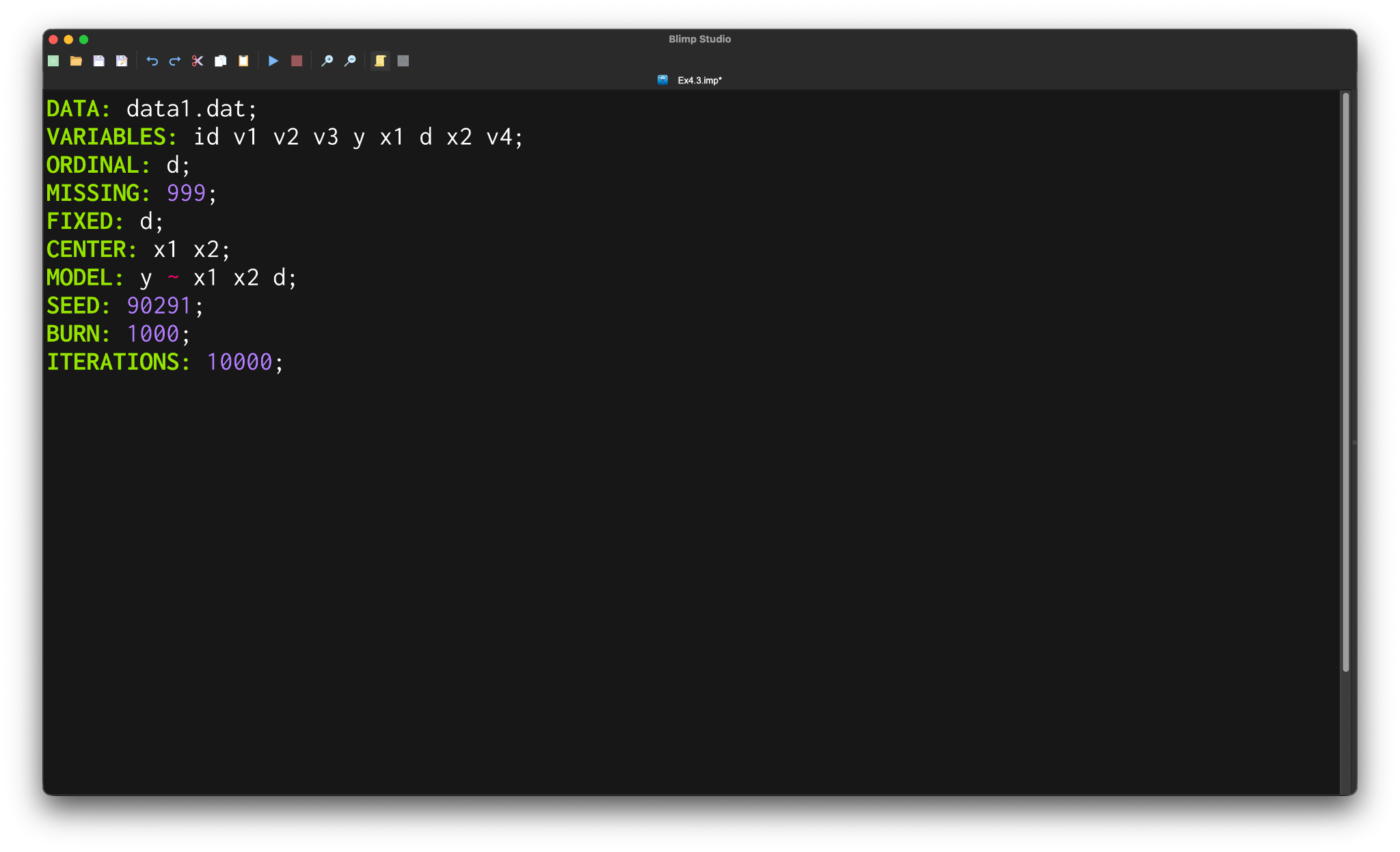
The Blimp Studio application features a tabbed interface that makes it easy to work with multiple scripts and projects at the same time. The graphic below shows the Blimp Studio interface.
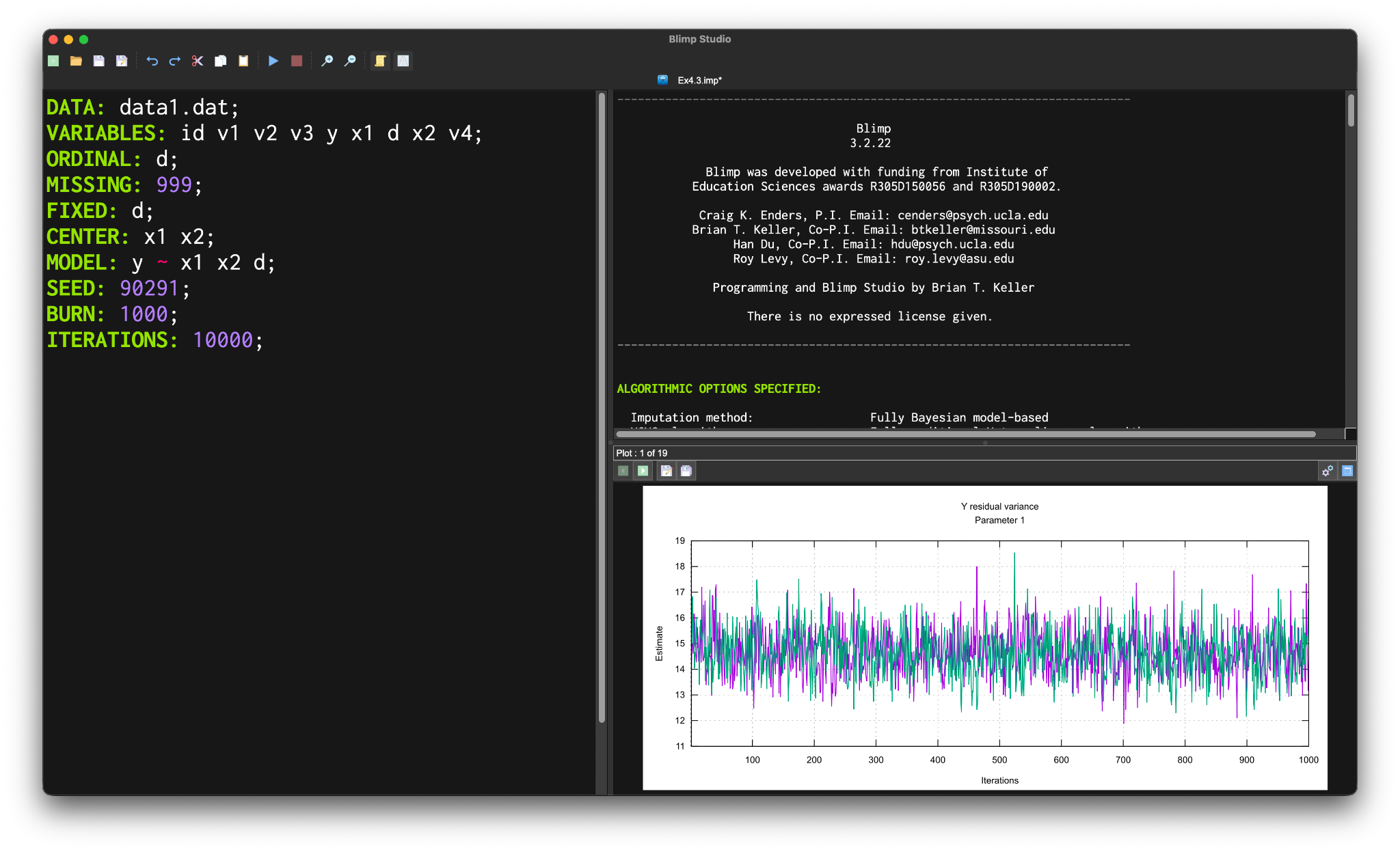
Clicking the blue arrow button on the toolbar executes a script and spawns a paned interface that adds an output window containing the analysis results and a plotting window displaying trace (time series) plots for every model parameter.
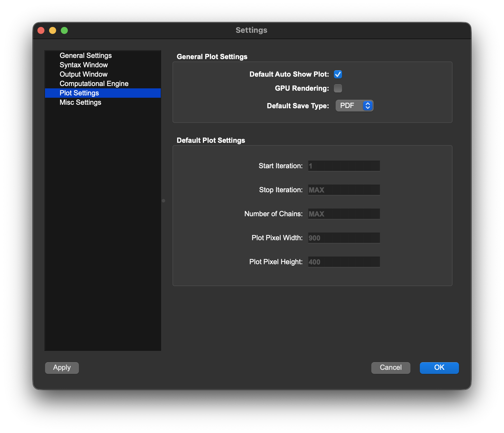
Clicking on the normal distribution icon in the toolbar hides the plotting window, which can also be disabled completely in the application’s Preferences, located under the Blimp Studio > Preferences pull-down menu. Other visual settings such as fonts and the orientation of the paned windows can also be set in the Preferences pane, shown below.
After executing a script in Blimp Studio, the output populates in the output pane (or R’s console window in rblimp). MCMC summary tables on Blimp’s output include unstandardized coefficients, standard deviations, standardized slopes, variances and covariances, and variance explained effect size estimates (Rights & Sterba, 2019). Certain types of analyses produce additional output (e.g., odds ratios in a logistic regression; transformation parameters for skewed variables). The graphic below shows a typical tabular display of the analysis results from a regression model. Blimp Studio automatically saves an output file with a .blimp-out extension to the same directory as the analysis script. The outputs are linked to their analysis scripts, such that double-clicking on one of the files opens both in the Blimp Studio interface.
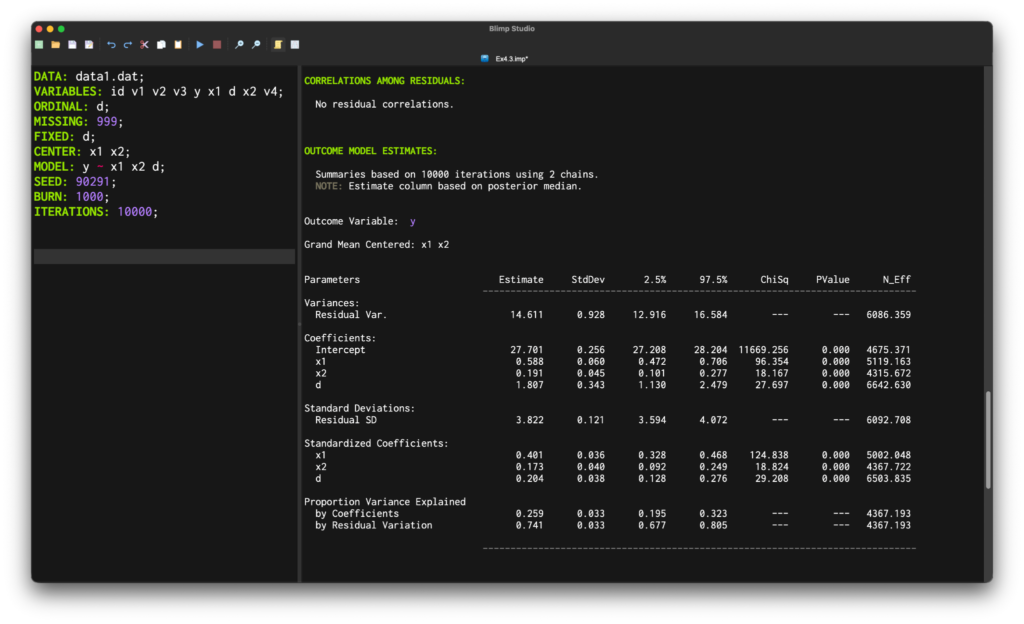
MCMC estimation produces a distribution for each model parameter. The estimate and standard deviation columns describe the center and spread of the posterior distributions; although they make no reference to drawing repeated samples, they are analogous—and numerically equivalent in most cases—to frequentist point estimates and standard errors. The 95% credible interval columns give a range that captures 95% of the parameter’s distribution. These are akin to confidence intervals, but the intervals describe parameter distributions rather than characteristics of repeated samples.
OUTCOME MODEL ESTIMATES:

  Summaries based on 10000 iterations using 2 chains.
  NOTE: Estimate column based on posterior median.

Outcome Variable:  y

Grand Mean Centered: x1 x2

Parameters                         Estimate     StdDev       2.5%      97.5%      ChiSq     PValue      N_Eff
                                ------------------------------------------------------------------------------
Variances:
  Residual Var.                      14.611      0.928     12.916     16.584        ---        ---   6086.359

Coefficients:
  Intercept                          27.701      0.256     27.208     28.204  11669.256      0.000   4675.371
  x1                                  0.588      0.060      0.472      0.706     96.354      0.000   5119.163
  x2                                  0.191      0.045      0.101      0.277     18.167      0.000   4315.672
  d                                   1.807      0.343      1.130      2.479     27.697      0.000   6642.630

Standard Deviations:
  Residual SD                         3.822      0.121      3.594      4.072        ---        ---   6092.708

Standardized Coefficients:
  x1                                  0.401      0.036      0.328      0.468    124.838      0.000   5002.048
  x2                                  0.173      0.040      0.092      0.249     18.824      0.000   4367.722
  d                                   0.204      0.038      0.128      0.276     29.208      0.000   6503.835

Proportion Variance Explained
  by Coefficients                     0.259      0.033      0.195      0.323        ---        ---   4367.193
  by Residual Variation               0.741      0.033      0.677      0.805        ---        ---   4367.193

                                ------------------------------------------------------------------------------
Although MCMC estimation is grounded in the Bayesian statistical paradigm, one can also view posterior medians, standard deviations, and credible intervals as surrogates for frequentist point estimates, standard errors, and confidence intervals. Levy and McNeish (2023) describe this perspective as “computational frequentism”. Essentially, the researcher wants to operate within the frequentist framework, but they use MCMC to solve a difficult estimation problem. Missing data analyses are a compelling use case for computational frequentism because optimal likelihood-based solutions are not always available or easy to use. To facilitate this perspective, the Blimp output also includes a chi-square statistic and p-value for each model parameter (the Bayesian Wald test; Asparouhov & Muthén, 2021). These Wald tests are like squared z–statistics from maximum likelihood estimation, but MCMC generates the point estimate and “standard error” for the test.
1.3 rblimp: Blimp in R
The rblimp package for R is currently available for download at CRAN or the blimp-stats GitHub. The most recent version of rblimp is available through GitHub, and CRAN updates are less frequent. The standalone version of Blimp must be installed prior to using rblimp, and the package installation process performs the install automatically.
The most recent version of rblimp is accessed on GitHub using the remotes package. Executing the commands shown below downloads and installs rblimp.
# install.packages('remotes')
remotes::install_github('blimp-stats/rblimp')
rblimp can be updated through CRAN or through GitHub by executing the following line of R code.
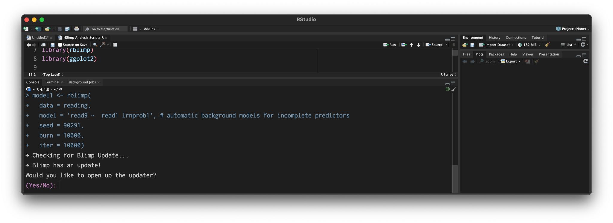
remotes::update_packages('rblimp')The Blimp Studio graphical interface automatically checks for updates each time the program is launched. Similarly, rblimp checks for updates to the computational engine and prompts the user to install. We recommend accepting these prompts, as the software is continually updated with new features.
When working in R, each Blimp command is simply an input parameter into the rblimp function. To illustrate, consider the following script from the GUI.
DATA: data1.dat;
VARIABLES: id n1 d1 o1 y x1 d2 x2 x3;
ORDINAL: d2;
MISSING: 999;
FIXED: d2;
CENTER: x1 x2;
MODEL: y ~ x1 d2 x2;
SEED: 90291;
BURN: 10000;
ITERATIONS: 10000;
The corresponding R script is as follows.
library(rblimp)
mymodel <- rblimp(
data = data,
ordinal = 'd2',
fixed = 'd2',
center = 'x1 x2',
model = 'y ~ x1 d2 x2',
seed = 90291,
burn = 10000,
iter = 10000
)
output(mymodel)
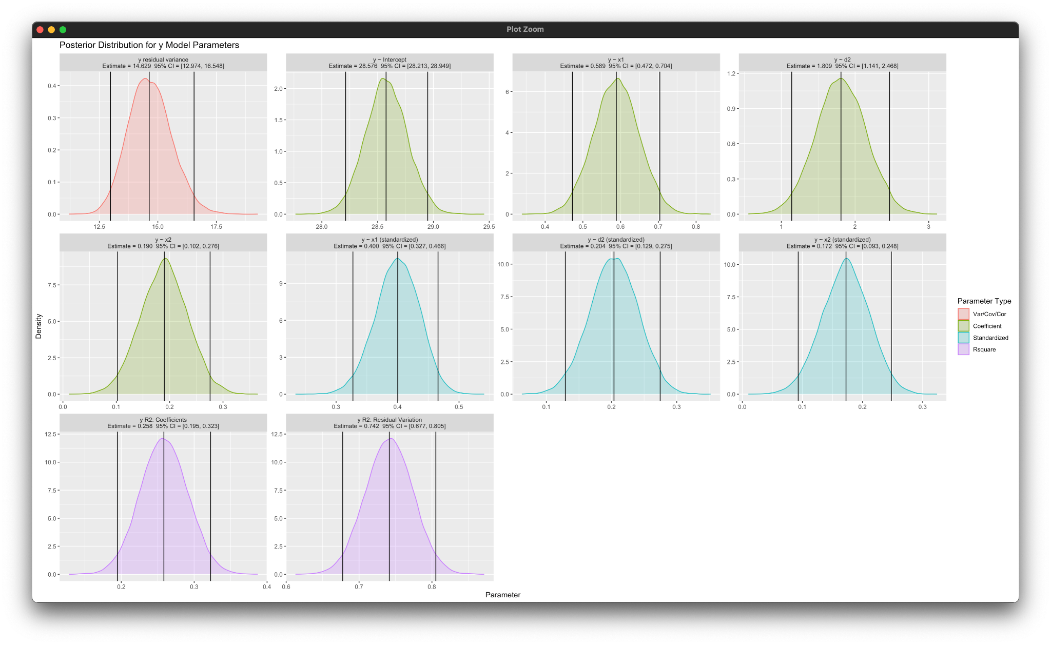
posterior_plot(mymodel, 'y')Each command in the Blimp script (each capitalized word) is an input parameter in the rblimp function. The three exceptions are the VARIABLES, MISSING, and SAVE commands. VARIABLES and MISSING are omitted because that information is contained in the R data file. The SAVE command is not needed because rblimp automatically saves all quantities computed during the MCMC process.
The rblimp package includes several plotting functions that are not available through the graphical interface. For example, the posterior_plot function produces graphical summaries of the model parameters, as shown below.
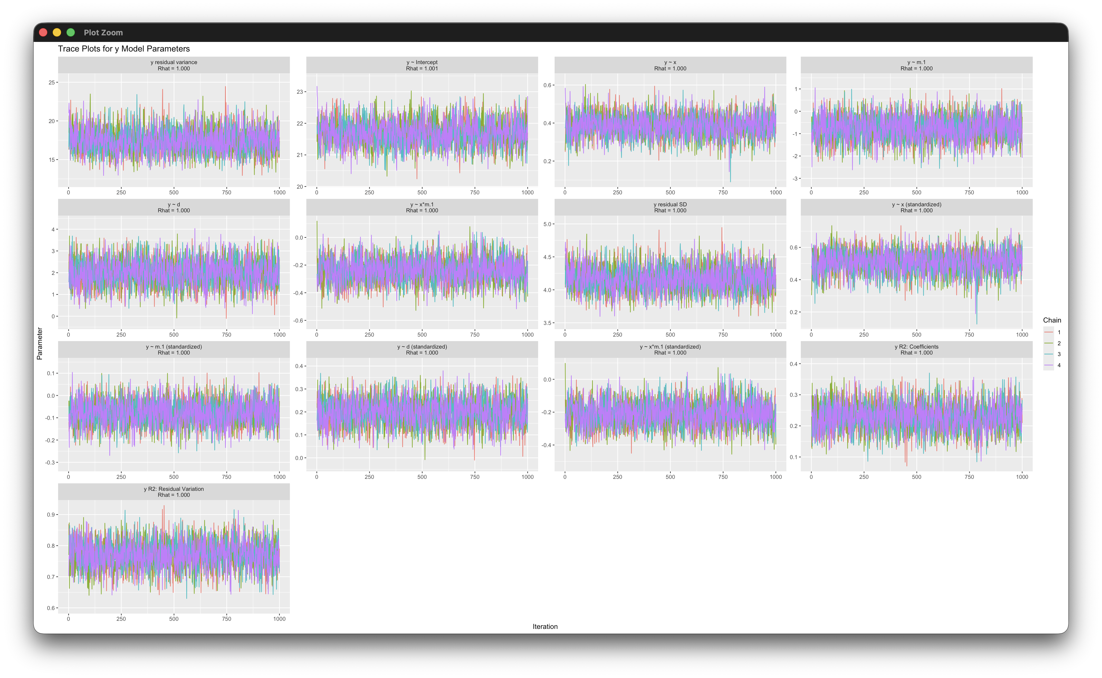
Similarly, the trace_plot function produces trace plots (line graphs) of parameter estimates. Chapter 3 illustrates this function.
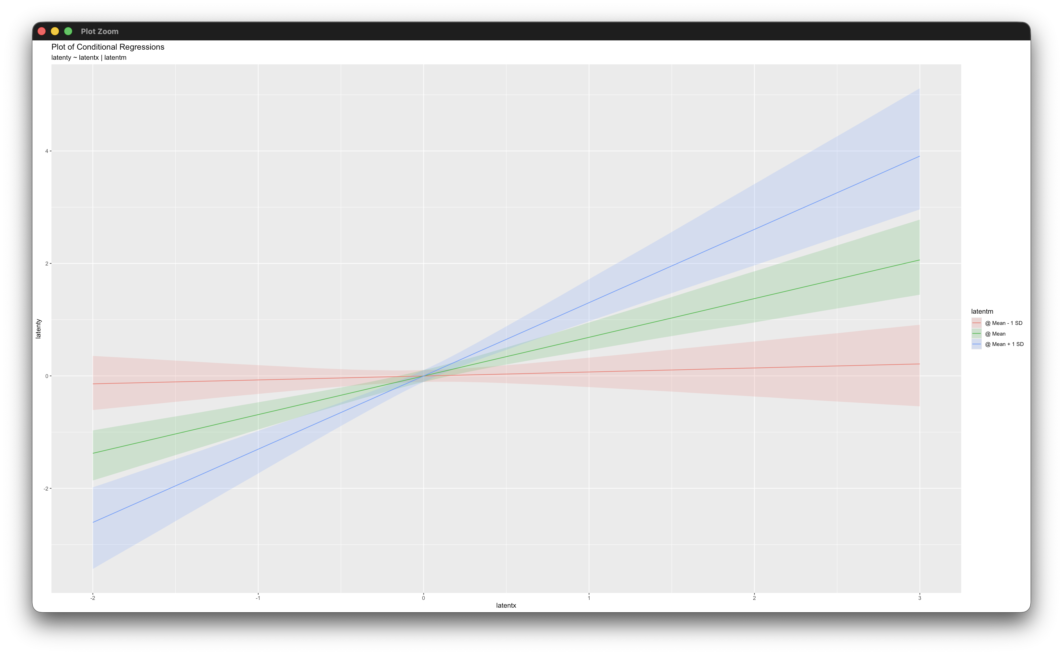
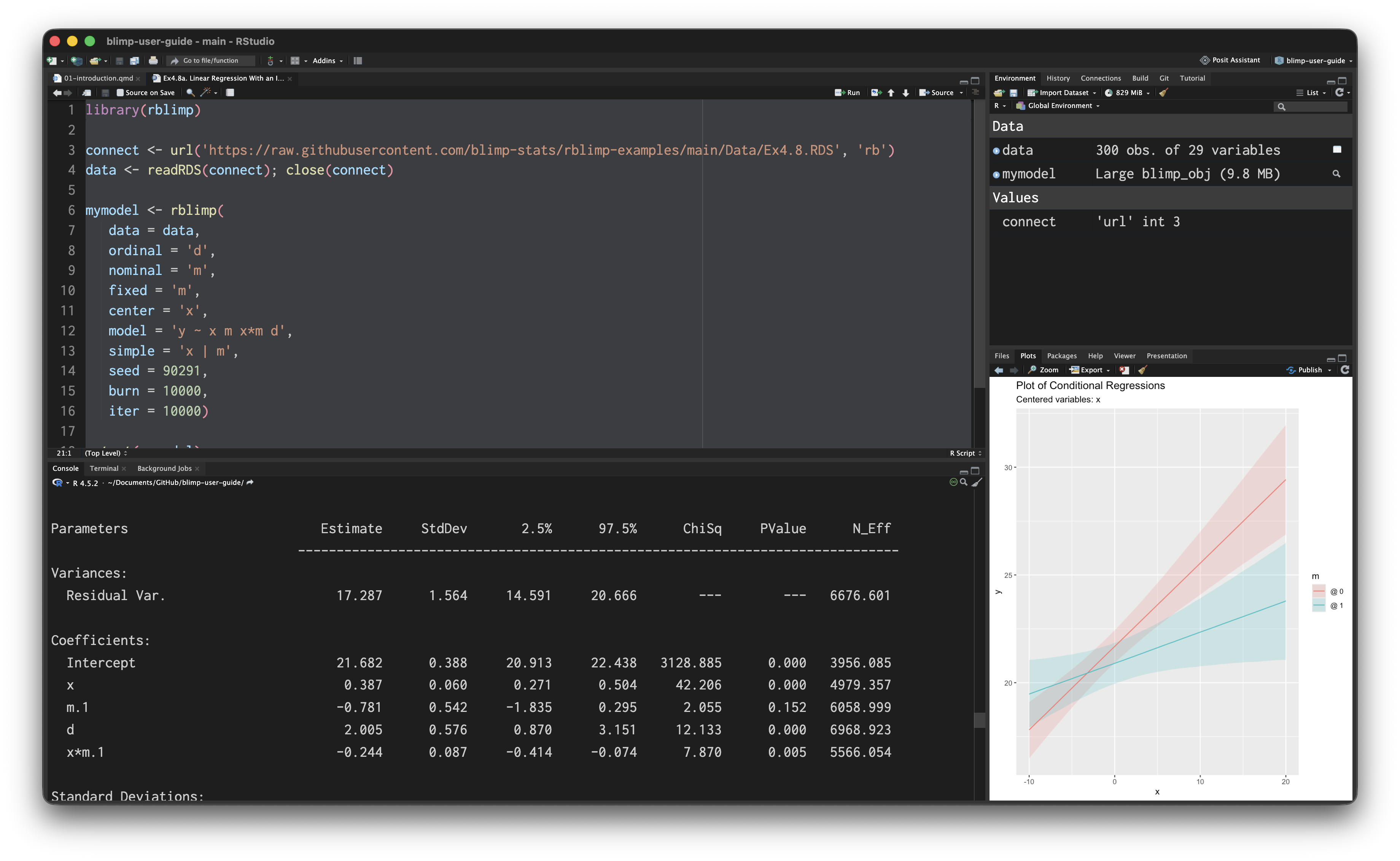
For models with interaction effects, the simple_plot function graphs conditional effects (simple intercepts and slopes), and the jn_plot function provides a graphical summary of the Johnson-Neyman technique for determining the values of the moderator that produce a significant conditional effect. The interaction plotting functions are illustrated in examples 4.8, 5.2, 5.13, 5.14, 5.15, 5.16, 6.15, and 6.16.
Following R convention, rblimp’s input parameters are separated by commas. Alphanumeric inputs like model statements, variable lists, transformations, and new parameters are enclosed in quotes. Numeric inputs like the seed and number of iterations do not require quotes. Finally, subcommands that are part of the same command (e.g., different equations in the MODEL command) are separated by semicolons, as they are in the Blimp Studio script.
model = '
   d2 ~ x2;
   x1 ~ d2 x2;
   y ~ x1 d2 x2;',
The standalone version of Blimp must be installed prior to downloading and installing rblimp because the R function calls the Blimp computational engine from the applications folder. Blimp otherwise behaves like any other package in the R environment.
All results that Blimp produces (estimates, MCMC samples, imputations, diagnostics, etc.) are automatically saved in the rblimp model object. Saved quantities can be inspected by typing @ after the model object’s name in the R console. For example, multiple imputations are saved in a list accessed by mymodel@imputations. Other saved quantities include: @estimates (table of all printed parameter values), @burn (MCMC estimates from burn-in iterations), @iterations (MCMC estimates for analysis iterations), @psr (potential scaled reduction diagnostics), @average_imp (average imputations across all MCMC iterations), @variance_imp, @waldtest, @syntax, and @output. Several examples from later chapters show how to analyze multiple imputations directly within R (see Examples 4.6, 4.7, 4.9, 5.10, 6.2, and 6.3).
1.4 Blimp’s Modeling Framework
The major feature that distinguishes Blimp’s estimation architecture from other latent variable modeling software packages is that it does not work with the joint distribution of the analysis variables. Rather, the multivariate distribution is factored into the product of multiple univariate distributions. A paper detailing Blimp’s “factored structural equation modeling” framework is available here.
To illustrate a factored specification, consider an analysis involving y, x, and m. The trivariate distribution factors into the product of three univariate distributions, each of which corresponds to a univariate regression model.
\[f\left(y,x,m\right)=f\left(y\middle| x,m\right)\times f\left(x\middle| m\right)\times f\left(m\right)\]
Blimp estimates the models on the right of the equals sign without assuming anything about the form or shape of the multivariate distribution on the left. The advantage of this specification is that the individual regression equations can feature mixtures of categorical and normal variables, continuous variables with skewed distributions, interactive or nonlinear terms, and other complex constructions. In such cases, the multivariate distribution on the left doesn’t have a known or simple form, and model misspecifications (e.g., treating such data as multivariate normal) can introduce bias.
The theory for Blimp’s model specification is given by Ibrahim and colleagues (Ibrahim, Chen, & Lipsitz, 2002; Ibrahim, Lipsitz, & Chen, 1999; Lipsitz & Ibrahim, 1996), and the software extends these ideas to latent variable models with up to three levels. More recent literature refers to this model specification as fully Bayesian estimation, the sequential specification, and factored regression (Enders et al., 2020; Erler, Rizopoulos, Jaddoe, Franco, & Lesaffre, 2019; Erler et al., 2016; Lüdtke, Robitzsch, & West, 2020a, 2020b; Zhang & Wang, 2017).
To illustrate Blimp’s modeling framework more concretely, consider a research scenario where the focal analysis model is a linear regression of y on x and m. The factorization above translates into the following linear regression models, where all residuals are normal and have constant variance.
\[y=\beta_0+\beta_1x_i+\beta_2m_i+\varepsilon_i\]
\[x_i=\gamma_{01}+\gamma_{11}m_i+r_{1i}\]
\[m_i=\gamma_{02}+r_{2i}\]
The x and m equations are essentially nuisance models in this example, and their role is to link incomplete predictors to one another as well as to any complete regressors.
Any univariate equation can feature mixtures of categorical and normal variables, continuous variables with skewed distributions, and interactive or nonlinear terms, among other things. For example, the following equations include an interaction between x and m in the focal model and a quadratic association between x and m in the supporting predictor model.
\[y=\beta_0+\beta_1x+\beta_2m+\beta_3(x)(m)+\varepsilon\]
\[x=\gamma_{01}+\gamma_{11}m+\gamma_{21}m^2+r_1\]
\[m=\gamma_{02}+r_2\]
If either x or m has missing values, a joint modeling framework is inappropriate and would produce biased estimates because the incomplete predictor distributions are complicated nonlinear functions of the outcome; such associations are fundamentally incompatible with off-the-shelf distributions such as the multivariate normal (Bartlett, Seaman, White, & Carpenter, 2015; Liu, Gelman, Hill, Su, & Kropko, 2014). Specifying a model as a sequence of factored regressions bypasses the problematic joint distribution altogether. These ideas readily extend to latent variables, which Blimp views as missing data to be estimated (imputed).
Blimp factorizations rely on three types of submodels: univariate distributions for outcome variables, multivariate distributions for manifest predictor variables, and multivariate distributions for correlated outcomes. To illustrate, consider the following path diagram, which features all three types.

Symbolically, the factorization for this model is as follows.
\[f\left(y,m_1,m_2,x_1,x_2\right)=f\left(y\middle| m_1,m_2,x_1,x_2\right)\times f\left(m_1,m_2\middle| x_1,x_2\right)\times f\left(x_1,x_2\right)\]
Virtually any model can be specified with some combination of these three distribution types. Importantly, the software constructs the appropriate factorization with no input from the user. To reiterate, distributional assumptions enter via three submodels, and Blimp makes no assumption about the form or shape of the joint distribution on the left side of the equation.
The symbolic representations have been intentionally vague because each \(f(\cdot)\) can represent different types of distributions. The table below summarizes the available variable types for each of Blimp’s three submodels.
| Variable Type | Outcomes (Univariate) |
Exogenous Predictors (Multivariate) |
Correlated Outcomes (Multivariate) |
|---|---|---|---|
| Normal manifest | ✓ | ✓ | ✓ |
| Normal latent | ✓ | ✓ | |
| Nonnormal manifest | ✓ (Yeo–Johnson) | ✓ (Yeo–Johnson) | |
| Nonnormal latent | ✓ (Yeo–Johnson) | ✓ (Yeo–Johnson) | |
| Binary | ✓ (logit or probit) | ✓ (probit) | ✓ (probit) |
| Ordinal | ✓ (probit) | ✓ (probit) | ✓ (probit) |
| Multicategorical | ✓ (logit) | ✓ (probit) | |
| Count | ✓ (negative binomial) | ||
| Two-Part | ✓ (any type) | ✓ (any type) |
Univariate outcome models (e.g., y) provide options that span most applications, including normal and nonnormal continuous variables (manifest or latent), common discrete outcomes (binary, ordinal, multicategorical, and count), and two-part models for floor and ceiling effects. The two multivariate submodels also allow various combinations of continuous and discrete variables. Exogenous predictor variables (e.g., x1 and x2) can be normal, binary, ordinal, or multicategorical. Finally, correlated outcomes (e.g., m1 and m2) can include mixtures of continuous (normal and skewed), binary, and ordinal variables. Generalized linear models for discrete outcomes use a latent response variable formulation. For skewed continuous variables, Blimp implements the Yeo–Johnson normalizing transformation.
1.5 Specifying Models for Incomplete Predictors
Throughout the guide, we use the term “predictors” to refer to exogenous variables—in a path diagram, variables that do not have incoming arrows. When predictors are complete, there is usually no reason to specify a distribution for these variables. Instead, the covariate data essentially function as known constants, as in ordinary least squares. In contrast, incomplete predictors require an explicit distribution for imputation. Blimp allows these distributions to have many forms (e.g., normal, skewed, discrete). In most cases, assigning a distribution to a predictor means making that regressor a dependent variable in its own regression model. These supporting models can be explicitly specified, or Blimp can create them automatically. These two strategies are somewhat different and have different strengths and weaknesses. We use the following multiple regression to illustrate the two model specification strategies, and we assume that all variables are incomplete.
\[y=\ \beta_0+\beta_1x_1+\beta_2x_2+\beta_3x_3+\varepsilon\]
To begin, consider the situation where Blimp automatically constructs supporting regression models for the predictors. The MODEL statement is as follows.
MODEL: y ~ x1 x2 x3;Throughout the guide, we refer to this specification as reflecting unspecified associations among the predictors. Blimp automatically adopts a two-part factorization that invokes a distribution for the outcome and another supporting multivariate submodel for the predictors. This default factorization for this example is as follows.
\[f\left(y, x_1, x_2, x_3\right) = f\left(y \middle| x_1, x_2, x_3\right) \times f\left(x_1, x_2, x_3\right)\]
We refer to this setup as a partially factored specification because it leaves the rightmost term—a multivariate normal distribution for continuous predictors and latent response variables—unfactored.
Algorithmically, the multivariate distribution for the predictors is represented as a round robin pattern where each predictor is regressed on all other predictors. These regressions exist for missing data handling and do not have a substantive interpretation. When all predictors are complete, Blimp automatically omits the supporting submodel for the predictors.
\[x_1=\mu_1+\gamma_{11}\left(x_2-\mu_2\right)+\gamma_{21}\left(x_3-\mu_3\right)+r_1\]
\[x_2=\mu_2+\gamma_{12}\left(x_1-\mu_1\right)+\gamma_{22}\left(x_3-\mu_3\right)+r_2\]
\[x_3=\mu_3+\gamma_{13}\left(x_1-\mu_1\right)+\gamma_{23}\left(x_2-\mu_2\right)+r_3\]
The regressions above are linear and assume normally distributed residuals, but this specification also allows for binary, ordinal, and multicategorical nominal predictors, in which case Blimp adopts a latent response variable formulation (Albert & Chib, 1993; Carpenter & Kenward, 2013; Enders et al., 2018; Johnson & Albert, 1999). Variable metrics are specified using the ORDINAL and NOMINAL commands described in Chapter 2. Enders et al. (2020) describe the multilevel version of this specification. The round robin regression equations above simplify missing data imputation by leveraging the property that a multivariate normal distribution spawns an equivalent set of linear regression models (Arnold, Castillo, & Sarabia, 2001; Liu, Gelman, Hill, Su, & Kropko, 2014). Importantly, the normal distribution assumption precludes the possibility of nonlinear associations among the predictors, as such relations are incompatible with normal data.
Next, consider the situation where the user explicitly specifies the regression equations for the predictors. This specification leverages the probability chain rule to factorize the joint distribution of the analysis variables into the product of several univariate conditional distributions, each of which corresponds to a regression model.
\[f\left(y,x_1,x_2,x_3\right)=f\left(y|x_1,x_2,x_3\right)\times f\left(x_1|x_2,x_3\right)\times\]
\[f\left(x_2\middle| x_3\right)\times f\left(x_3\right)\]
The corresponding regression equations follow the same cascading pattern where the first predictor’s model is empty, the second predictor is regressed on the first, the third on the first and second, and so on.
\[x_1=\gamma_{01}+\gamma_{11}x_2+\gamma_{21}x_3+r_1\]
\[x_2=\gamma_{02}+\gamma_{12}x_3+r_2\]
\[x_3=\gamma_{03}+r_3\]
The MODEL statement for this specification is
MODEL:
  predictor.models:
  x3 ~ 1;
  x2 ~ x3;
  x1 ~ x2 x3;
  focal.model:
  y ~ x1 x2 x3;
and the code block below illustrates a syntax shortcut for this specification that lists all predictors to the left of a tilde.
MODEL:
  predictor.models:
  x1 x2 x3 ~ 1;
  focal.model:
  y ~ x1 x2 x3;
We refer to this setup as a sequential specification (Erler et al., 2016; Lüdtke et al., 2020b).
Blimp’s output produces a tabular summary for each estimated model (there are four in the previous example). By default, the summary tables are alphabetized according to the outcome’s name. Some users may prefer to order the tables so the primary analysis results appear first. This is accomplished by using labels ending in a colon to define blocks of models that appear in the order listed. The following example creates two model blocks, such that the focal model summary table appears first on the printed output.
MODEL:
  focal.model:
  y ~ x1 x2 x3;
  predictor.models:
  x1 x2 x3 ~ 1;
The sequential specification for predictors differs in important ways. First, the predictor’s equation can have any metric allowed by Blimp—normal, skewed continuous, binary (probit or logit link), ordinal (probit link), multicategorical nominal (logistic link), or count (negative binomial link). Second, associations among the predictors need not be linear. For example, the following equations include the quadratic effect of x3 on x2.
\[x_1=\gamma_{01}+\gamma_{11}x_2+\gamma_{21}x_3+r_1\]
\[x_2=\gamma_{02}+\gamma_{12}x_3+\gamma_{22}x_3^2+r_2\]
\[x_3=\gamma_{03}+r_3\]
The corresponding MODEL statement is as follows.
MODEL:
  predictor.models:
  x3 ~ 1;
  x2 ~ x3 (x3^2);
  x1 ~ x2 x3;
  focal.model:
  y ~ x1 x2 x3;
When using a sequential specification, ordering the predictors in a particular way can facilitate estimation and reduce the impact of model misspecifications. Lüdtke et al. (2020b, pp. 171-172) recommend ordering variables from left to right by their missingness rates, with categorical variables before continuous variables. To illustrate, suppose that x1 is an incomplete binary variable, x2 is complete, and x3 is an incomplete continuous variable. Their recommended specification would be as follows
\[f\left(y|x_1,x_2,x_3\right)\times f\left(x_3|x_1,x_2\right)\times f\left(x_1|x_2\right)\times f\left(x_2\right)\]
and the corresponding model specification is
ORDINAL: x1;
MODEL:
  predictor.models:
  x2 ~ 1;
  x1 ~ x2;
  x3 ~ x1 x2;
  focal.model:
  y ~ x1 x2 x3;
or simply as follows.
ORDINAL: x1;
MODEL:
  predictor.models:
  x3 x1 x2 ~ 1;
  focal.model:
  y ~ x1 x2 x3;
Finally, when predictors are complete, there is usually no reason to specify a distribution for these variables; instead, the covariate data essentially function as known constants, as in ordinary least squares. With either specification for the predictors, listing complete predictors on the FIXED command line indicates that the variable does not require a model (or distribution). Continuing with the previous example where x2 is complete, the sequential specification moves the complete variable from the left to the right of the tilde, as follows.
FIXED: x2;
MODEL:
  predictor.models:
  x3 x1 ~ x2;
  focal.model:
  y ~ x1 x2 x3;
The partially factored specification with unspecified predictor associations is as follows.
FIXED: x2;
MODEL: y ~ x1 x2 x3;
The examples in Chapters 4 through 7 generally treat predictor distributions as unspecified. This setup is easy to specify, and it is also convenient for centering because the means are explicit model parameters that MCMC iteratively estimates. This approach does not limit the composition of the focal analysis model, which can include interactive or nonlinear terms. However, predictor regressions are necessarily additive, as interactions and similar nonlinearities are incompatible with a multivariate normal distribution. As mentioned previously, unspecified predictor associations accommodate normal, binary, ordinal, and multicategorical variables via a latent response variable framework. Blimp can apply a Yeo–Johnson (Yeo & Johnson, 2000) distribution to skewed variables and negative binomial regression to count variables, but these features require a sequential specification.
1.6 Missing Data Handling
As detailed in Sections 1.4 and 1.5, Blimp’s estimation architecture factorizes a multivariate distribution into the product of univariate distributions. This factorization carries through to missing data handling, where the distributions of missing values rely on a collection of univariate models. The advantage of this specification is that Blimp can generate appropriate imputations from models that are fundamentally incompatible with known multivariate distributions. Examples include models with incomplete interactive or polynomial effects, multilevel models with random effects, and models with skewed variables or mixtures of discrete and numeric variables.
To illustrate missing data handling, consider an analysis involving y, x, and m. To refresh, the trivariate distribution factors into the product of three univariate distributions, each of which corresponds to a regression model.
\[f\left(y,x,m\right)=f\left(y\middle| x,m\right)\times f\left(x\middle| m\right)\times f\left(m\right)\]
Blimp estimates the models on the right of the equals sign without assuming anything about the form or shape of the multivariate distribution on the left. In a simple scenario where all three three variables are continuous, the factorization corresponds to the following linear regression models.
\[y=\beta_0+\beta_1x_i+\beta_2m_i+\varepsilon_i\]
\[x_i=\gamma_{01}+\gamma_{11}m_i+r_{1i}\]
\[m_i=\gamma_{02}+r_{2i}\]
In a factored regression framework, the distributions of missing values depend on every model in which a variable appears. For example, the distribution of missing y values depends only on the analysis model, and MCMC samples imputations from a normal curve with center and spread equal to a predicted value and residual variance, respectively.
\[f\left(y|x,m\right)=N\left(\beta_0+\beta_1x_i+\beta_2m_i,\sigma_\varepsilon^2\right)\]
Because it appears in two models—once as a predictor and once as an outcome—the conditional distribution of missing x values is proportional to the product of two normal distributions.
\[\begin{aligned} f\left(x|y,m\right) &\propto f\left(y\middle| x,m\right)\times f\left(x\middle| m\right) \\ &= N\left(\beta_0+\beta_1x_i+\beta_2m_i,\sigma_\varepsilon^2\right)\times N\left(\gamma_{01}+\gamma_{11}m_i,\sigma_{r1}^2\right) \end{aligned}\]
In a similar vein, the conditional distribution of the missing m values is proportional to the product of three normal distributions.
\[\begin{aligned} f\left(m\middle| y,x\right) &\propto N\left(\beta_0+\beta_1x_i+\beta_2m_i,\sigma_\varepsilon^2\right)\times N\left(\gamma_{01}+\gamma_{11}m_i,\sigma_{r1}^2\right) \\ &\quad \times N\left(\gamma_{02},\sigma_{r2}^2\right) \end{aligned}\]
These conditional distributions have analytic solutions in many cases (Levy & Enders, 2021), but Blimp’s MCMC algorithm uses Metropolis sampling to draw imputations from composite functions such as these.
With a collection of additive models like those above, the distributions of missing values are equivalent to the distributions implied by a joint modeling framework or fully conditional specification. The same is not true for models with nonlinearities, skewed variables, or mixtures of discrete and numeric variables. To illustrate, suppose the analysis model includes an interaction between x and m. The factorization and the corresponding regression models are as follows.
\[f\left(y,x,m\right)\propto f\left(y\middle| x,m,x\times m\right)\times f\left(x\middle| m\right)\times f\left(m\right)\]
\[y=\beta_0+\beta_1x_i+\beta_2m_i+\beta_3\left(x_i\times m_i\right)+\varepsilon\]
\[x_i=\gamma_{01}+\gamma_{11}m_i+r_{1i}\]
\[m_i=\gamma_{02}+r_{2i}\]
As before, the distributions of missing values depend on every model in which a variable appears. For example, the distribution of missing x values is again the product of two normal distributions, as follows.
\[\begin{aligned} f\left(x|y,m\right) &\propto f\left(y\middle| x,m,x\times m\right)\times f\left(x\middle| m\right) \\ &= N\left(\beta_0+\beta_1x_i+\beta_2m_i+\beta_3\left(x_i\times m_i\right),\sigma_\varepsilon^2\right) \\ &\quad \times N\left(\gamma_{01}+\gamma_{11}m_i,\sigma_{r1}^2\right) \end{aligned}\]
Importantly, the conditional distribution of missing values is incompatible with multivariate normality because its variance is heteroscedastic function (Enders et al., 2020, Eq. 8). The same issue applies more broadly to models with polynomial or nonlinear terms and multilevel models with random effects, among others.
Basing imputations on factored regression specification is guaranteed to produce a set of compatible univariate regressions, whereas conventional modeling frameworks that create imputations based on a multivariate distribution are prone to bias (Bartlett, Seaman, White, & Carpenter, 2015; Liu, Gelman, Hill, Su, & Kropko, 2014). More generally, the univariate models described above could feature discrete variables (binary, ordinal, multicategorical nominal, count), skewed continuous variables, and even latent variables, which Blimp views as missing data to be estimated (imputed).
1.7 Prior Distributions
Blimp’s MCMC algorithm adopts different prior distributions that depend on the variable’s metric and the type of model. Blimp invokes a normal distribution prior for regression coefficients (and means). We denote these priors as normal(mu, var). The default noninformative prior is a normal distribution with infinite variance. Variances and residual variances use a conjugate inverse gamma prior distribution. The inverse gamma distribution has two parameters, scale and shape. We denote this distribution as invgamma(a,b). The scale parameter can be viewed as the prior degrees of freedom ÷ 2, and the shape parameter is the prior sums of squares ÷ 2. For covariance matrices, Blimp adopts conjugate inverse Wishart priors. The inverse Wishart distribution is the multivariate extension of the inverse gamma. It too has two parameters, a scale matrix and degrees of freedom. We denote this prior as IW(SSp,dfp), where SSp is the prior sum of squares and cross-products matrix (the scale matrix), and dfp is the prior degrees of freedom. In the table below, we use p to denote the number of variance in the covariance matrix. The table below summarizes the default prior distributions, and the rightmost column indicates whether the user can specify a custom prior. Priors are modified using either the OPTIONS command or the PARAMETERS command.
| Variable Type | Parameter | Default Prior | Modifiable |
|---|---|---|---|
| Continuous exogenous manifest predictors with unspecified associations | Regression coefficients | normal(0,Inf) | No |
| Continuous exogenous manifest predictors with unspecified associations | Residual variance | invgamma(1,.5) | Yes ( OPTIONS command) |
| Ordinal exogenous manifest predictor (> two categories) | Threshold | uniform(–Inf,Inf) | No |
| Discrete exogenous manifest predictor | Residual variance | NA (fixed parameter) | NA |
| Continuous outcome (manifest or latent) | Regression coefficients | normal(0,Inf) | Yes (PARAMETERS command) |
| Continuous outcome (manifest or latent) | Residual variance | invgamma(–1,0) | Yes (OPTIONS and PARAMETERS commands) |
| Discrete outcome | Regression coefficients | normal(0,5) | Yes (PARAMETERS command) |
| Discrete outcome | Residual variance | NA (fixed parameter) | NA |
| Ordinal outcome (> two categories) | Threshold | uniform(–Inf,Inf) | No |
| Random effect residual in a mixed model | Covariance matrix | IW(0,–p–1) | Yes ( OPTIONS command) |
| Continuous outcome (manifest, latent, or binary/ordinal latent response variables) | Covariance matrix | IW(0,–p–1) | Yes ( OPTIONS command) |
1.8 New Features
The following is a list of new features and functionality available in Version 4.
- Up to a 2x to 3x speed increase from version 3
- R integration with rblimp on CRAN
- Multilevel models with dynamic lagged effects (DSEM)
- Residualized effects (RSEM) for analyses like the random intercept cross-lagged panel model
- Skewed latent variables using the Yeo–Johnson transformation
- Location–scale multilevel models
- Easier specification of selection models and pattern mixture models for MNAR missingness processes, including MNAR models for multilevel data
- Convenience features like definition variables and looping structures for specifying complex models
- Enhanced data simulation features
The following is a list of features and functionality that were introduced in Version 3.2.
- Multiple-equation models (e.g., path models) with up to three levels
- Latent variables and latent variable regressions
- Latent variables with random effects, interactions, and nonlinear effects
- Single-level and multilevel selection and pattern mixtures models for missing not at random processes
- Multivariate regression models
- Parameter constraints
- Auxiliary parameters that are functions of estimated parameters
- Latent variable imputation
- Yeo–Johnson modeling for skewed continuous variables
- Binary and multinomial logistic regression
- Negative binomial regression for count outcomes
- Estimation with sampling weights
- Facilities for computing new variables with numerous built-in functions
- Built-in functions embedded within regression equations
- Facilities for introducing custom univariate prior distributions
- New Blimp Studio graphical user interface
- Redesigned output with numerous enhancements and additional printing options
- Better optimization and many algorithmic improvements
- Enhanced user guide with dozens of new examples and analysis scripts
- Enhanced WALDTEST command for Bayesian Wald tests in all models Blimp estimates
- DIC and WAIC information criteria for model selection
- Correlations among the residuals of all outcome variables for evaluating local sources of model misfit
The following is a list of features and functionality that were introduced in Version 2.
- WALDTEST command for Bayesian Wald tests (Asparouhov & Muthén, 2021)
- Simplified scripting language and redesigned output
- Graphical interface with automatic updates when new features become available
- Graphical engine that creates trace plots for all model parameters
- Bayesian estimation of single-level, multilevel (up to three levels), and multiple group regression models with complete or incomplete data
- Posterior summaries of all model parameters from Bayesian estimation (posterior mean, median, standard deviation, and credible interval)
- Single-level and multilevel R-squared measures (Rights & Sterba, 2019)
- Bayesian estimation for interactive and nonlinear effects with missing data
- Bayesian estimation with grand mean centering (all models) and group mean centering (two- and three-level models)
- Post-hoc probing of interaction effects with continuous or categorical moderators
- Bayesian estimation of conditional effects (simple slopes) in regression models with interaction effects
- Incomplete binary, ordinal, or nominal predictor variables
- Discrete and latent imputations for binary, ordinal, and nominal variables
- FCS or Bayesian estimation with level-2 and level-3 cluster means modeled as latent variables
- Contextual effects models with latent group means or manifest group means
- Interaction effects with latent group means
- Various algorithmic and interface enhancements (eg, random starting values, options for saving various estimates and output)
1.9 Running From Terminal
Blimp scripts can also be executed from the terminal without the graphical interface. This is useful when conducting computer simulations, for example. The most basic specification includes a file path to the Blimp executable file followed by a file path to the script to be executed. To illustrate, the following line of code executes a script located on the desktop.
/Applications/Blimp/blimp ~/desktop/myscript.impSimilarly, the following line uses the Blimp beta engine to execute the same file.
/Applications/Blimp/blimp-beta ~/desktop/myscript.impSeveral parts of the Blimp script can be specified via command line arguments. The general form of an argument includes a double dash followed by a keyword and an input parameter. For example, the following code block uses a command line argument to specify the input data set.
BLIMPPATH=/Applications/Blimp/blimp
${BLIMPPATH} ~/desktop/myscript.imp --data ~/desktop/mydata.dat
Note that any parameters specified as command line arguments replace the current contents of the script (e.g., the file specified on the DATA command is replaced by the file ~/desktop/mydata.dat).
In addition to the input data, command line arguments include the random number seed and most quantities exported using the SAVE command. The code block below shows the full array of command line arguments. The backslash is the Linux command continuation character; the arguments would otherwise need to appear on a single line separated by a space.
/Applications/Blimp/blimp ~/desktop/myscript.imp \
   --seed {seed value} \
   --data {filepath to input data} \
   --output {filepath to blimp-out output file} \
   --stacked {filepath to stacked imputation data} \
   --stacked0 {filepath to stacked original + imputed data} \
   --separate {filepath to separate imputation data sets} \
   --estimates {filepath to save estimate summary tables} \
   --burn {filepath to save all burn-in estimates} \
   --iterations {filepath to save all post burn-in estimates} \
   --psr {filepath to save burn-in psr values} \
   --waldtest {filepath to save Wald statistics} \