7 Missing Not at Random Process Examples

This section illustrates missing not at random analysis models in Blimp. Following previous chapters, the examples in this section use a generic notation system where variable names usually consist of an alphanumeric prefix and a numeric suffix (e.g., y, x1, x2, n1, d1, d2). The letter y designates a dependent variable, a d prefix denotes a binary dummy variable, an o prefix indicates an ordinal variable, and an n prefix indicates a multicategorical nominal variable. Additionally, the multilevel examples use a “_i” suffix to denote level-1 variables, “_j” for level-2 variables, and “_k” for level-3 variables (e.g., d_j is a level-2 dummy variable, x_i is a continuous predictor measured at level-1). Blimp determines the levels automatically, so the suffixes are meant as a visual aid for understanding the scripts. Finally, the model equations use “c” and “w” superscripts to indicate grand and group mean centering, respectively. The following list outlines the examples in this section.

7.1: Selection Model for Linear Regression
7.2: Pattern Mixture Model for Linear Regression
7.3: Shared Parameter (Wu–Carroll) Latent Curve Model
7.4: Diggle–Kenward Latent Curve Model
7.5: Factor Analysis With a Selection Model
7.6: Mediation Analysis With a Selection Model
7.7: Two-Level Hedeker-Gibbons Pattern Mixture Growth Model
7.8: Selection Model for a Two-Level Regression With Random Coefficients
7.9: Two-Level Shared Parameter Growth Curve Model
7.10: Two-Level Diggle–Kenward Growth Curve Model

7.1 Selection Model for Linear Regression

This example illustrates a selection model for a missing not at random process where an incomplete outcome variable predicts its own missingness. The focal analysis model is the linear regression below. The c superscript denotes variables centered at their grand means.

\[y=\beta_0+\beta_1d_{1}+\beta_2d_2+\beta_3x_{1}^{c}+\varepsilon\]

The most basic selection model is one where the outcome alone predicts its missingness indicator (m = 0 if y is observed and 1 if it’s missing); Gomer and Yuan (2021) refer to this as a focused missing not at random process. The following equation is a probit model where the missingness indicator’s latent response variable (denoted by an asterisk superscript) is regressed on the outcome.

\[m_{y}^\ast=\gamma_0+\gamma_1y+r\]

For identification, the residual variance is fixed at one, and the threshold parameter is fixed at zero. A path diagram of the model is shown below.

The analysis model also incorporates three auxiliary variables using the sequential specification from Example 4.7. The full set of User Guide examples is available from the Examples pull-down menu in the Blimp Studio graphical interface. A GitHub repository with Blimp Studio scripts and data is available here, and a repository containing the rblimp scripts is available here.

The syntax highlights are listed below. Adding the NIMPS and SAVE commands generates model-based multiple imputations for a frequentist analysis that no longer requires a missingness model.

ORDINAL command identifies binary predictors
FIXED command identifies complete predictors (optional—speeds computation)
CENTER command applies grand mean centering to predictors
MODEL command uses labels ending in a colon to group models and order their summary tables on the output
MODEL command features a syntax shortcut that creates a factored regression (sequential) specification for auxiliary variables
The .missing suffix references the dependent variable’s missing data indicator, which is automatically defined as ordinal
Unspecified associations for predictor variables

DATA: data3.dat;
VARIABLES: id x1 x2 x3 y d1 d2 v1:v4;
MISSING: 999;
ORDINAL: d1 d2;
FIXED: d1 d2;
CENTER: x1;
MODEL:
  focal.model:
  y ~ d1 d2 x1;
  missingness.model:
  y.missing ~ y;
  auxiliary.model:
  x2 x3 ~ y d1 d2 x1;
SEED: 90291;
BURN: 10000;
ITER: 10000;

The corresponding rblimp script is as follows.

library(rblimp)

mymodel <- rblimp(
  data = data,
  ordinal = 'd1 d2',
  fixed = 'd1 d2',
  center = 'x1',
  model = '
    focal.model:
    y ~ d1 d2 x1;
    missingness.model:
    y.missing ~ y;
    auxiliary.model:
    x2 x3 ~ y d1 d2 x1',
  seed = 90291,
  burn = 10000,
  iter = 10000
)

output(mymodel)

A more complex selection model features the outcome predicting its missingness indicator along with other variables, in this case d1; Gomer and Yuan (2021) refer to this as a diffuse missing not at random process. The following equation is a probit model where the missingness indicator’s latent response variable is regressed the outcome and d1.

\[m_{y}^\ast=\gamma_0+\gamma_1y+\gamma_2d_{1}+r\]

A path diagram of the model is shown below.

Caution is warranted when including too many predictors from the analysis model in the selection equation, as doing so weakens identification. Entering and selecting predictors in a stepwise fashion using fit indices such as the DIC and WAIC is often a good strategy. The code block for the analysis is shown below.

DATA: data3.dat;
VARIABLES: id x1 x2 x3 y d1 d2 v1:v4;
MISSING: 999;
ORDINAL: d1 d2;
FIXED: d1 d2;
CENTER: x1;
MODEL:
  # focal analysis model
  y ~ d1 d2 x1;
  # auxiliary variable models
  x2 x3 ~ y d1 d2 x1;
  # selection model
  y.missing ~ y d1;
SEED: 90291;
BURN: 10000;
ITER: 10000;

The corresponding rblimp script is as follows.

library(rblimp)

mymodel <- rblimp(
  data = data3,
  ordinal = 'd1 d2',
  fixed = 'd1 d2',
  center = 'x1',
  model = '
    y ~ d1 d2 x1;
    x2 x3 ~ y d1 d2 x1;
    y.missing ~ y d1',
  seed = 90291,
  burn = 10000,
  iter = 10000
)

output(mymodel)

7.2 Pattern Mixture Model for Linear Regression

This example illustrates a pattern mixture model for a missing not at random process where regression model parameters differ between cases with and without dependent variable scores. The focal analysis model is the linear regression below

\[y=\beta_0+\beta_1d_{1}+\beta_2d_2+\beta_3x_{1}^{c}+\varepsilon\]

where d1 is a dummy code representing a focal group comparison (e.g., a treatment assignment indicator), and d2 and x1 are covariates. The c superscript denotes variables centered at their grand means.

The most basic pattern mixture model is one where the intercept (outcome variable mean) differs between people with and without y values; Gomer and Yuan (2021) characterize this as a focused missing not at random process. The fitted model features a binary missing data indicator (m = 0 if y is observed and m = 1 if it’s missing) as a predictor, as follows.

\[y=\beta_{0(obs)}+\beta_{0(diff)}m_{y}+\beta_1d_{1}+\beta_2d_{2}+\beta_3x_{1}^{c}+\varepsilon\]

A path diagram of the model is shown below.

The overall population-level intercept estimate is a weighted average of the pattern-specific intercepts, where the weights are the group proportions. The marginal intercept estimate for this example is

\[\beta_0=p_{(obs)}\beta_{0(obs)}+p_{(mis)}\beta_{0(mis)}=p_{(obs)}\beta_{0(obs)}+p_{(mis)}\left(\beta_{0(obs)}+\beta_{0(diff)}\right)\]

where p_(obs) and p_(mis) are the proportions of completers and dropouts, respectively.

Importantly, the intercept difference (the dashed line pointing from m to y) is inestimable because people in the m = 1 group have no data on y. This parameter must be fixed to a value during estimation, and the magnitude and sign of the coefficient controls the strength and direction of the missing not at random process. Enders (2022, Section 9.7) illustrates a strategy that uses off-the-shelf effect size benchmarks to determine this parameter. For example, if a researcher felt that the unseen y scores have a higher mean than the observed data, then the inestimable intercept coefficient could be solved as a function of the standardized mean difference effect size and the dependent variable’s standard deviation (or residual standard deviation).

\[\beta_{0(diff)}=d\times\sigma_y\]

A positive value of the effect size d sets the mean of the unseen scores to a higher value than the observed data, and a negative value specifies a lower mean. The code block below sets the effect size equal to +0.20 and uses the residual standard deviation to estimate the spread of y (Little, 2009, p. 428). This setting corresponds to a sensitivity analysis where persons with incomplete data are hypothesized to have a mean difference roughly equal to Cohen’s (1988) small effect size benchmark.

The full set of User Guide examples is available from the Examples pull-down menu in the Blimp Studio graphical interface. A GitHub repository with Blimp Studio scripts and data is available here, and a repository containing the rblimp scripts is available here.

The syntax highlights are listed below. Adding the NIMPS and SAVE commands generates model-based multiple imputations for a frequentist analysis that no longer requires the missing data indicator.

ORDINAL command identifies binary predictors
FIXED command identifies complete predictors (optional—speeds computation)
CENTER command applies grand mean centering to predictors
MODEL command uses labels ending in a colon to group models and order their summary tables on the output
MODEL command features a syntax shortcut that creates a factored regression (sequential) specification for all predictor
MODEL command features a syntax shortcut that creates a factored regression (sequential) specification for auxiliary variables
The TRANSFORM command creates the dependent variable’s missing data indicator, m.y
MODEL command labels the missing data indicator’s latent response variable mean and three parameters from the focal analysis model: the residual variance, intercept coefficient, and intercept mean difference
PARAMETERS command passes the value of the residual standard deviation into the formula that determines the intercept mean difference
PARAMETERS command uses labeled quantities to compute missing data group proportions, pattern-specific intercept coefficients, and a marginal intercept estimate that averages over the missing data patterns

DATA: data3.dat;
VARIABLES: id x1 x2 x3 y d1 d2 v1:v4;
MISSING: 999;
ORDINAL: d1 d2 ymis;
CENTER: x1;
TRANSFORM: ymis = ismissing(y);
MODEL:
  focal.model:
  y ~ 1@b0obs ymis@b0diff d1 d2 x1;
  # label residual variance
  y@resvar;
  predictor.model:
  # sequential specification for predictors
  ymis ~ 1@ymissmean;
  x1 d1 d2 ~ ymis;
  auxiliary.model:
  x2 x3 ~ y d1 d2 x1;
PARAMETERS:
  # set b0diff equal to +.20 residual std. dev. units
  cohensd = .20;
  b0diff = cohensd * sqrt(resvar);
  # missingness group proportions
  p_mis = phi(ymissmean);
  p_obs = 1 - p_mis;
  # compute weighted average intercept
  b0_obs = b0obs;
  b0_mis = b0obs + b0diff;
  b0 = (b0_obs * p_obs) + (b0_mis * p_mis);
SEED: 90291;
BURN: 10000;
ITER: 10000;

The corresponding rblimp script is as follows.

library(rblimp)

mymodel <- rblimp(
  data = data,
  ordinal = 'd1 d2 ymis',
  center = 'x1',
  transform = 'ymis = ismissing(y)',
  model = '
    focal.model:
    y ~ 1@b0obs ymis@b0diff d1 d2 x1 ;
    y@resvar;
    predictor.model:
    ymis ~ 1@ymissmean;
    x1 d1 d2 ~ ymis;
    auxiliary.model:
    x2 x3 ~ y d1 d2 x1',
  parameters = '
    cohensd = .20;
    b0diff = cohensd * sqrt(resvar);
    p_mis = phi(ymissmean);
    p_obs = 1 - p_mis;
    b0_obs = b0obs;
    b0_mis = b0obs + b0diff;
    b0 = (b0_obs * p_obs) + (b0_mis * p_mis)',
  seed = 90291,
  burn = 10000,
  iter = 10000
)

output(mymodel)
posterior_plot(mymodel)

A more complex pattern mixture model is one where people with missing outcome scores have different intercepts and slopes than people with data; Gomer and Yuan (2021) characterize this as a diffuse missing not at random process. The fitted model features the missing data indicator and its interaction with the focal predictor, d1.

\[y=\beta_{0(obs)}+\beta_{0(diff)}m_{y}+\beta_{1(obs)}d_{1}+\beta_{1(diff)}(d_{1}\times m_{y})+ \beta_2d_{2}+\beta_3x_{1}^{c}+\varepsilon\]

A path diagram of the model is as follows.

The marginal slope that averages over the missing data patterns is a weighted average of the pattern-specific slopes, with weights equal to the group proportions.

\[\beta_1=p_{(obs)}\beta_{1(obs)}+p_{(mis)}\beta_{1(mis)}=p_{(obs)}\beta_{1(obs)}+p_{(mis)}\left(\beta_{1(obs)}+\beta_{1(diff)}\right)\]

Importantly, both the intercept and slope difference for the incomplete cases (the dashed lines pointing from m to y and m to d1’s slope) are inestimable because people in the m = 1 group have no data on y. As such, these parameters must be fixed to a value during estimation, and their magnitude and sign control the strength and direction of the missing not at random process. The same effect size-based strategy can be applied to the slope difference. In this example, the focal predictor d1 is binary (e.g, intervention vs. control), in which case β_1(obs) is the group mean difference for people with data on y, and β_1(diff) is the additional group mean difference for persons with missing y scores. Specifying the inestimable slope as a standardized mean difference effect size gives the following solution.

\[\beta_{1(diff)}=d\times\sigma_y\]

If the focal predictor is continuous, then the solution is

\[\beta_{1(diff)}=d\times\left(\sigma_y\div\sigma_x\right)\]

in which case the d effect size can be viewed as the additional change in the dependent variable (in standard deviation units) for every one standard deviation increase in the predictor. Setting d to a positive value means that the missing data group’s slope is more positive, and a negative value of d means their slope is more negative.

To illustrate, suppose that y is scaled such that high scores reflect a negative outcome (e.g., greater illness severity, a higher symptom count), and d1 is a treatment assignment dummy code (d1 = 0 indicates the control group, and d1 = 1 is the intervention group). Further, consider a missing not at random process where control group participants with the highest y scores (e.g., most acute symptoms) leave the study to seek treatment elsewhere, whereas intervention group participants with the lowest y scores (e.g., mildest symptoms) leave the study because they no longer feel treatment is necessary. This scenario requires a positive value of d for the inestimable intercept difference and a negative value of d for the slope difference. The code block below sets both effect sizes equal to 0.20 (they need not be the same) and uses the residual standard deviation to estimate the spread of y.

DATA: data3.dat;
VARIABLES: id x1 x2 x3 y d1 d2 v1:v4;
MISSING: 999;
ORDINAL: d1 d2 m.y;
TRANSFORM:
  m.y = ismissing(y);
CENTER: x1;
MODEL:
  focal.model:
  y ~ 1@b0obs m.y@b0diff d1@b1obs d1*m.y@b1diff d2 x1;
  # label residual variance
  y ~~ y@resvar;
  predictor.model:
  m.y ~ 1@ymissmean;
  x1 d1 d2 ~ m.y;
  auxiliary.model:
  x2 x3 ~ y x1 d1 d2;
PARAMETERS:
  # set b0diff equal to +.20 residual std. dev. units
  # set b1diff equal to -.20 residual std. dev. units
  cohensd = .20;
  b0diff = cohensd * sqrt(resvar);
  b1diff = - cohensd * sqrt(resvar);
  # missingness group proportions
  p.mis = phi(ymissmean);
  p.obs = 1 - p.mis;
  # compute weighted average intercept and slope
  b0.obs = b0obs;
  b0.mis = b0obs + b0diff;
  b1.obs = b1obs;
  b1.mis = b1obs + b1diff;
  b0 = (b0.obs * p.obs) + (b0.mis * p.mis);
  b1 = (b1.obs * p.obs) + (b1.mis * p.mis);
SEED: 90291;
BURN: 10000;
ITER: 10000;

The corresponding rblimp script is as follows.

library(rblimp)

mymodel <- rblimp(
  data = data,
  ordinal = 'd1 d2 m.y',
  transform = 'm.y = ismissing(y)',
  center = 'x1',
  model = '
    focal.model:
    y ~ 1@b0obs m.y@b0diff d1@b1obs d1*m.y@b1diff d2 x1;
    y@resvar;
    predictor.model:
    m.y ~ 1@ymissmean;
    x1 d1 d2 ~ m.y;
    auxiliary.model:
    x2 x3 ~ y x1 d1 d2',
  parameters = '
    cohensd = .20;
    b0diff = cohensd * sqrt(resvar);
    b1diff = - cohensd * sqrt(resvar);
    p.mis = phi(ymissmean);
    p.obs = 1 - p.mis ;
    b0.obs = b0obs;
    b0.mis = b0obs + b0diff;
    b1.obs = b1obs;
    b1.mis = b1obs + b1diff;
    b0 = (b0.obs * p.obs) + (b0.mis * p.mis);
    b1 = (b1.obs * p.obs) + (b1.mis * p.mis)',
  seed = 90291,
  burn = 10000,
  iter = 10000
)

output(mymodel)
posterior_plot(mymodel)

Linking inestimable parameters to the standardized mean difference provides a practical heuristic for specifying inestimable coefficients, but it is still incumbent on the researcher to choose values that are reasonable for a given application. As mentioned previously, the magnitude of the missing data group’s difference parameters dictates the strength of the missing not at random process. It is incorrect to view “small” values of d as unimportant, as standardized differences of this magnitude could be very salient in many situations. For example, consider a randomized intervention where the true effect size is d = 0.20 (i.e., a small effect size). Setting the missing data group’s coefficient difference to d = .20 means that the moderating impact of missing data is just as large as the intervention effect itself. A medium effect size threshold is probably an upper bound for most practical applications, and much smaller values of d could be realistic. A sensitivity analysis strategy would examine the changes in the focal model parameters across a range of d values (see Enders 2022, Section 9.8).

7.3 Shared Parameter (Wu–Carroll) Latent Curve Model

This example illustrates a two-factor latent growth curve model with the Wu–Carroll (1988) model for missing not at random dropout that depends on the growth trajectories. A path diagram of the model is shown below.

The model features binary dropout indicators (m2 to m6) regressed on the random intercepts and slopes. The indicators are denoted as ovals to convey that the outcomes are latent response variables (probit regression).

Importantly, the missing data indicators code attrition or permanent dropout rather than intermittent missingness. Accordingly, the m variables equal 0 prior to dropout, 1 at the occasion participants leave the study, and 999 (missing) at all post-dropout measurements. There is no dropout indicator for y1 because this variable is complete. The path coefficients connecting dropout at occasion t to the random intercepts are constrained to equality, as are the coefficients connecting the random slopes to dropout. The dashed lines convey these constraints. Predictor variables can be incorporated into either the outcome or dropout part of the model. Additional details about this model can be found in Enders (2011) and Muthén, Asparouhov, Hunter, and Leuchter (2011).

The syntax highlights are as follows.

ORDINALcommand identifies the binary dropout indicators
LATENT command defines two latent variables
MODEL command uses labels ending in a colon to group models and order their summary tables on the output
Individual regression equations specified for each indicator (instead of the -> convention for latent factors)
MODEL command uses the -> convention to add random intercepts and slopes as a predictor to each measurement model and fix the loadings and measurement intercepts
MODEL command uses a label to impose equality constraint on residual variance, a label to constrain associations between the random intercepts and indicators, and a label to constrain associations between the random slopes and indicators

DATA: data24.dat;
VARIABLES: id y1 y2 y3 y4 y5 y6 m1 m2 m3 m4 m5 m6;
ORDINAL: m2:m6;
MISSING: 999;
LATENT: eta_icept eta_slope;
MODEL:
  structural.model:
  eta_icept ~ 1;
  eta_slope ~ 1;
  eta_icept ~~ eta_slope;
  measurement.model:
  eta_icept -> y1@1 y2@1 y3@1 y4@1 y5@1 y6@1;
  eta_slope -> y1@0 y2@1 y3@2 y4@3 y5@4 y6@5;
  1 -> y1@0 y2@0 y3@0 y4@0 y5@0 y6@0;
  y1@vconstraint;
  y2@vconstraint;
  y3@vconstraint;
  y4@vconstraint;
  y5@vconstraint;
  y6@vconstraint;
  dropout.model:
  m2 ~ eta_icept@iconstraint eta_slope@sconstraint;
  m3 ~ eta_icept@iconstraint eta_slope@sconstraint;
  m4 ~ eta_icept@iconstraint eta_slope@sconstraint;
  m5 ~ eta_icept@iconstraint eta_slope@sconstraint;
  m6 ~ eta_icept@iconstraint eta_slope@sconstraint;
SEED: 90291;
BURN: 100000;
ITER: 100000;

The corresponding rblimp script is as follows.

library(rblimp)

mymodel <- rblimp(
  data = data,
  ordinal = 'm2:m6',
  latent = 'eta_icept eta_slope',
  model = '
    structural.model:
    eta_icept ~ 1;
    eta_slope ~ 1;
    eta_icept ~~ eta_slope;
    measurement.model:
    eta_icept -> y1@1 y2@1 y3@1 y4@1 y5@1 y6@1;
    eta_slope -> y1@0 y2@1 y3@2 y4@3 y5@4 y6@5;
    1 -> y1@0 y2@0 y3@0 y4@0 y5@0 y6@0;
    y1@vconstraint;
    y2@vconstraint;
    y3@vconstraint;
    y4@vconstraint;
    y5@vconstraint;
    y6@vconstraint;
    dropout.model:
    m2 ~ eta_icept@iconstraint eta_slope@sconstraint;
    m3 ~ eta_icept@iconstraint eta_slope@sconstraint;
    m4 ~ eta_icept@iconstraint eta_slope@sconstraint;
    m5 ~ eta_icept@iconstraint eta_slope@sconstraint;
    m6 ~ eta_icept@iconstraint eta_slope@sconstraint;',
  seed = 90291,
  burn = 100000,
  iter = 100000
)

output(mymodel)
posterior_plot(mymodel)

7.4 Diggle-Kenward Latent Curve Model

This example illustrates a two-factor latent growth curve model with the Diggle–Kenward (1994) model for missing not at random dropout that depends on the unseen outcome score at time t. A path diagram of the model is shown below.

The model features binary dropout indicators (m2 to m6) regressed on the repeated measurements. The indicators are denoted as ovals to convey that the outcomes are latent response variables (probit regression).

Importantly, the missing data indicators code attrition or permanent dropout rather than intermittent missingness. Accordingly, the m variables equal 0 prior to dropout, 1 at the occasion participants leave the study, and 999 (missing) at all post-dropout measurements. There is no dropout indicator for y1 because this variable is complete. The path coefficients connecting dropout at occasion t to the observed data from the previous occasion are constrained to equality, as are the paths connecting dropout at occasion t with the concurrent (unseen) scores at occasion t. The dashed lines convey these constraints. Predictor variables can be incorporated into either the outcome or dropout part of the model. Additional details about this model can be found in Enders (2011) and Muthén, Asparouhov, Hunter, and Leuchter (2011).

The syntax highlights are as follows.

ORDINALcommand identifies the binary dropout indicators
LATENT command defines two latent variables
MODEL command uses labels ending in a colon to group models and order their summary tables on the output
Individual regression equations specified for each indicator (instead of the -> convention for latent factors)
MODEL command uses the -> convention to add random intercepts and slopes as a predictor to each measurement model and fix the loadings and measurement intercepts
MODEL command uses a label to impose equality constraint on residual variance, a label to constrain lagged associations between the outcomes and indicators, and a label to constrain concurrent associations between the outcomes and indicators
Longer burn-in period for estimating latent variables

DATA: data23.dat;
VARIABLES: id y1 y2 y3 y4 y5 y6 m1 m2 m3 m4 m5 m6;
ORDINAL: m2:m6;
MISSING: 999;
LATENT: eta_icept eta_slope;
MODEL:
  structural.model:
  eta_icept ~ 1;
  eta_slope ~ 1;
  eta_icept ~~ eta_slope;
  measurement.model:
  eta_icept -> y1@1 y2@1 y3@1 y4@1 y5@1 y6@1;
  eta_slope -> y1@0 y2@1 y3@2 y4@3 y5@4 y6@5;
  1 -> y1@0 y2@0 y3@0 y4@0 y5@0 y6@0;
  y1 ~~ y1@vconstraint;
  y2 ~~ y2@vconstraint;
  y3 ~~ y3@vconstraint;
  y4 ~~ y4@vconstraint;
  y5 ~~ y5@vconstraint;
  y6 ~~ y6@vconstraint;
  dropout.model:
  m2 ~ y1@marconstraint y2@mnarconstraint;
  m3 ~ y2@marconstraint y3@mnarconstraint;
  m4 ~ y3@marconstraint y4@mnarconstraint;
  m5 ~ y4@marconstraint y5@mnarconstraint;
  m6 ~ y5@marconstraint y6@mnarconstraint;
SEED: 90291;
BURN: 100000;
ITER: 100000;

The corresponding rblimp script is as follows.

library(rblimp)

mymodel <- rblimp(
  data = data,
  ordinal = 'm2:m6',
  latent = 'eta_icept eta_slope',
  model = '
    structural.model:
    eta_icept ~ 1;
    eta_slope ~ 1;
    eta_icept ~~ eta_slope;
    measurement.model:
    eta_icept -> y1@1 y2@1 y3@1 y4@1 y5@1 y6@1;
    eta_slope -> y1@0 y2@1 y3@2 y4@3 y5@4 y6@5;
    1 -> y1@0 y2@0 y3@0 y4@0 y5@0 y6@0;
    y1 ~~ y1@vconstraint;
    y2 ~~ y2@vconstraint;
    y3 ~~ y3@vconstraint;
    y4 ~~ y4@vconstraint;
    y5 ~~ y5@vconstraint;
    y6 ~~ y6@vconstraint;
    dropout.model:
    m2 ~ y1@marconstraint y2@mnarconstraint;
    m3 ~ y2@marconstraint y3@mnarconstraint;
    m4 ~ y3@marconstraint y4@mnarconstraint;
    m5 ~ y4@marconstraint y5@mnarconstraint;
    m6 ~ y5@marconstraint y6@mnarconstraint;',
  seed = 90291,
  burn = 100000,
  iter = 100000
)

output(mymodel)
posterior_plot(mymodel)

7.5 Factor Analysis With a Selection Model

This example illustrates a two-factor measurement model with correlated latent variables, each measured by six continuous indicators. A path diagram of the analysis model is shown in Section 5.7. The main difference is that the analysis incorporates a selection missingness model for the indicators of one latent factor. The selection equations model a missing not at random process where missingness is explained by an individual’s standing on the latent trait. A path diagram of the model is shown below.

The m variables are binary missing data indicators coded 0 if a response is complete and 1 if missing. The path coefficients connecting the missingness indicators to the latent factor are constrained to equality (i.e., one’s standing on the factor exerts the same influence on the probability of missing not at random missingness). The dashed lines convey these constraints.

The syntax highlights are as follows.

LATENT command defines two latent variables
TRANSFORM command uses the ismissing function to create missing data indicators for the six y items
MODEL command uses labels ending in a colon to group models and order their summary tables on the output
MODEL command uses a label to impose equality constraint on the associations between the latent factor and the missingness indicators
MODEL command fixes variances and residual variances to one for identification
PARAMETERS command specifies a truncated prior over positive values, and the prior is attached to each factor’s first loading in the MODEL command

DATA: data4.dat;
VARIABLES: id v1:v9 y1:y6 v10:v16 x1:x6;
MISSING: 999;
ORDINAL: m1:m6;
TRANSFORM:
  m1 = ismissing(y1);
  m2 = ismissing(y2);
  m3 = ismissing(y3);
  m4 = ismissing(y4);
  m5 = ismissing(y5);
  m6 = ismissing(y6);
LATENT: latenty latentx;
MODEL:
  latent.model:
  latentx@1;
  latenty@1;
  latentx ~~ latenty;
  measurement.models:
  latentx -> x1@xload_prior x2:x6;
  latenty -> y1@yload_prior y2:y6;
  missingness.model:
  m1 ~ latenty@misconstraint;
  m2 ~ latenty@misconstraint;
  m3 ~ latenty@misconstraint;
  m4 ~ latenty@misconstraint;
  m5 ~ latenty@misconstraint;
  m6 ~ latenty@misconstraint;
PARAMETERS:
  xload_prior ~ truncate(0, Inf);
  yload_prior ~ truncate(0, Inf);
SEED: 90291;
BURN: 20000;
ITER: 20000;

The corresponding rblimp script is as follows.

library(rblimp)

mymodel <- rblimp(
  data = data,
  ordinal = 'm1:m6',
  transform = '
    m1 = ismissing(y1);
    m2 = ismissing(y2);
    m3 = ismissing(y3);
    m4 = ismissing(y4);
    m5 = ismissing(y5);
    m6 = ismissing(y6);',
  latent = 'latenty latentx',
  model = '
    latent.model:
    latentx@1;
    latenty@1;
    latentx ~~ latenty;
    measurement.models:
    latentx -> x1@xload_prior x2:x6;
    latenty -> y1@yload_prior y2:y6;
    missingness.model:
    m1 ~ latenty@misconstraint;
    m2 ~ latenty@misconstraint;
    m3 ~ latenty@misconstraint;
    m4 ~ latenty@misconstraint;
    m5 ~ latenty@misconstraint;
    m6 ~ latenty@misconstraint',
  parameters = '
    xload_prior ~ truncate(0,Inf);
    yload_prior ~ truncate(0,Inf)',
  seed = 90291,
  burn = 20000,
  iter = 20000
)

output(mymodel)
posterior_plot(mymodel)

7.6 Mediation Analysis With a Selection Model

This example illustrates a single-mediator path model with selection models for a missing not at random process on the mediator and outcome. The focal regression models are shown below

\[m=I_m+{\alpha}x+\varepsilon_m\]

\[y=I_y+{\beta}m+{\tau}^{'}x+\varepsilon_y\]

where 𝛼 and 𝛽 are slope coefficients that define the indirect effect or product of the coefficients estimator, and 𝜏’ is the direct effect of x on y. A path diagram of the analysis is shown in Section 5.1. The analysis additionally incorporates missingness models for both m and y.

\[m_{m}^{*}=\gamma_{01}+\gamma_{11}m+\gamma_{21}x+\varepsilon_1\]

\[m_{y}^{*}=\gamma_{02}+\gamma_{12}y+\gamma_{22}m+\gamma_{32}x+\varepsilon_2\]

The asterisk superscripts on the binary missing data indicators represent latent response variables from a probit regression. m’s missingness model features m and x as predictors, and y’s missingness model features y, m, and x. Finally, the model also incorporates three auxiliary variables following the procedure from Example 4.7. A path diagram of the focal model is shown below.

The syntax highlights are as follows.

TRANSFORM command uses the ismissing function to create missing data indicators for m and y
MODEL command uses labels ending in a colon to group models and order their summary tables on the output
MODEL command labels the indirect effect’s component pathways
MODEL command features a syntax shortcut that creates a factored regression (sequential) specification for auxiliary variables
PARAMETERS command uses labeled quantities to compute the product of coefficients estimator

DATA: data4.dat;
VARIABLES: id a1:a3 v1 y m v2 x v3:v22;
MISSING: 999;
TRANSFORM:
  m.m = ismissing(m);
  m.y = ismissing(y);
MODEL:
  mediation.model:
  m ~ x@alpha;
  y ~ m@beta x;
  missingness.model:
  m.m ~ m x;
  m.y ~ y m x;
  auxiliary.model:
  a1:a3 ~ y m x;
PARAMETERS:
  indirect = alpha * beta;
SEED: 90291;
BURN: 10000;
ITER: 10000;

The corresponding rblimp script is as follows.

library(rblimp)

mymodel <- rblimp(
  data = data,
  transform = '
    m.m = ismissing(m);
    m.y = ismissing(y)',
  model = '
    mediation.model:
    m ~ x@alpha;
    y ~ m@beta x;
    missingness.model:
    m.m ~ m x;
    m.y ~ y m x;
    auxiliary.model:
    a1:a3 ~ y m x',
  parameters = 'indirect = alpha * beta',
  seed = 90291,
  burn = 10000,
  iter = 10000
)

output(mymodel)
posterior_plot(mymodel)
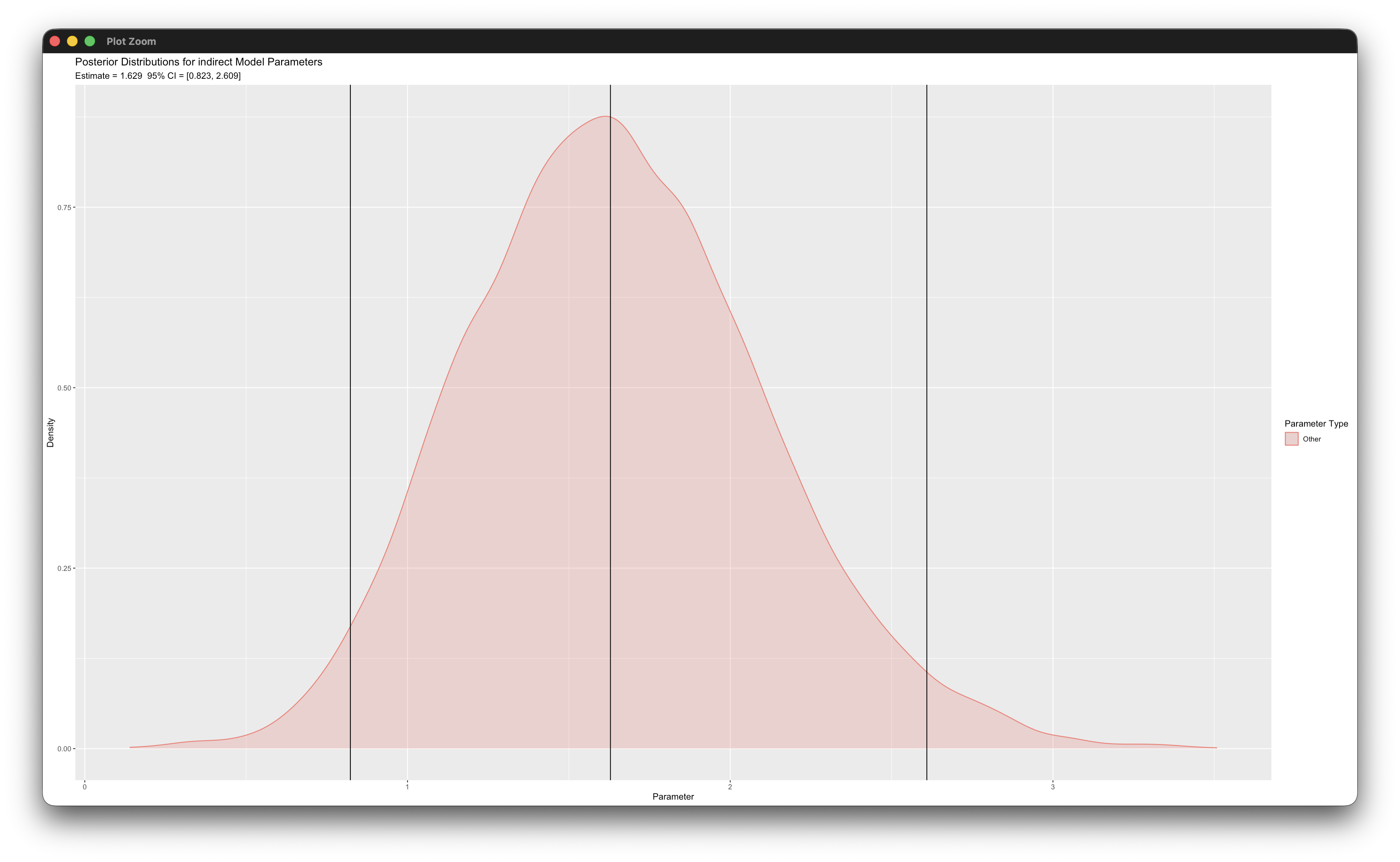
posterior_plot(mymodel,'indirect')

Working in rblimp is advantageous because graphing functions are available for visualizing results. For example, the second posterior_plot function call graphs the distribution of the mediated effect, which is named indirect. The 95% intervals are asymmetric because the distribution is skewed, and the graph indicates that the indirect effect is significant because zero is not within the interval.

7.7 Two-Level Hedeker-Gibbons Pattern Mixture Growth Model

This example illustrates the random coefficient pattern mixture model from Hedeker and Gibbons (1997). The model is designed for a missing not at random process where growth model parameters differ between cases who complete the study versus those who dropout. The multilevel model features a cross-level (group-by-time) interaction effect involving a level-2 dummy code d_j (e.g., a treatment assignment indicator) and the level-1 time scores, as follows.

\[y_{ij}=\left(\beta_0+b_{0j}\right)+\left(\beta_1+b_{1j}\right)({TIME}_{ij})+\beta_2(d_{j})+\beta_3\left({TIME}_{ij})(d_{j}\right)+\varepsilon_{ij}\]

The pattern mixture model introduces a dropout indicator that differentiates completers and dropouts, m_j = 0 and 1, respectively. The fitted model features the dropout indicator and its interaction effects

\[y_{ij}=\beta_{0(obs)}+\beta_{1(obs)}time_{ij}+\beta_{2(obs)}(d_{j})+\beta_{3(obs)}(time_{ij})(d_{j})\]

\[+\beta_{0(diff)}(m_j)+\beta_{1(diff)}(time_{ij})(m_j)+\beta_{2(diff)}(d_{j})(m_j )\]

\[+\beta_{3(diff)}(time_{ij})(d_{j})(m_j)+b_{0j}+b_{1j}(time_{ij})+\varepsilon_ij\]

where the “obs” subscript denotes the completer group’s (m_j = 0) parameters, and the “diff” subscript denotes coefficient differences for the dropout group (m_j = 1). Following Example 7.2, the overall population-level estimates (i.e., the marginal estimates that average over the distribution of missingness) are a weighted average of the pattern-specific coefficients, where the weights are the group proportions. The marginal estimates for this example are shown below, where p_(obs) and p_(mis) are the proportions of completers and dropouts, respectively.

\[\beta_0=p_{(obs)}\beta_{0(obs)}+p_{(mis)}\beta_{0(mis)}=p_{(obs)}\beta_{0(obs)}+p_{(mis)}\left(\beta_{0(obs)}+\beta_{0(diff)}\right)\]

\[\beta_1=p_{(obs)}\beta_{1(obs)}+p_{(mis)}\beta_{1(mis)}=p_{(obs)}\beta_{1(obs)}+p_{(mis)}\left(\beta_{1(obs)}+\beta_{1(diff)}\right)\]

\[\beta_2=p_{(obs)}\beta_{2(obs)}+p_{(mis)}\beta_{2(mis)}=p_{(obs)}\beta_{2(obs)}+p_{(mis)}\left(\beta_{2(obs)}+\beta_{2(diff)}\right)\]

\[\beta_3=p_{(obs)}\beta_{3(obs)}+p_{(mis)}\beta_{3(mis)}=p_{(obs)}\beta_{3(obs)}+p_{(mis)}\left(\beta_{3(obs)}+\beta_{3(diff)}\right)\]

The syntax highlights are listed below. Adding the NIMPS and SAVE commands generates model-based multiple imputations for a frequentist analysis (see Example 6.3).

CLUSTERID command identifies a level-2 identifier, automatically inducing random intercepts for all level-1 variables
ORDINAL command identifies binary predictors
CENTER command applies grand mean and latent group mean centering to predictors
MODEL command uses labels ending in a colon to group models and order their summary tables on the output
MODEL command features a random coefficient listed after the vertical pipe
MODEL command labels each fixed effect coefficient
MODEL command features a factored regression (sequential) specification for the binary predictors
PARAMETERS command uses labeled quantities to compute population-average (marginal) coefficients that average over missing data patterns

DATA: data18.dat;
VARIABLES: level2id v1_j d_j y_i time_i v2_j m_j v3_i;
ORDINAL: d_j m_j;
CLUSTERID: level2id;
MISSING: 999;
FIXED: time_i;
MODEL:
  focal.model:
  y_i ~ 1@beta0_obs time_i@beta1_obs d_j@beta2_obs
    (time_i*d_j)@beta3_obs m_j@beta0_dif (m_j*time_i)@beta1_dif
    (m_j*d_j)@beta2_dif (m_j*time_i*d_j)@beta3_dif | time_i;
  predictor.model:
  m_j ~ 1@ymissmean;
  d_j ~ m_j;
PARAMETERS:
  p_mis = phi(ymissmean);
  p_obs = 1 - p_mis ;
  beta0 = p_obs * beta0_obs + p_mis * (beta0_obs + beta0_dif);
  beta1 = p_obs * beta1_obs + p_mis * (beta1_obs + beta1_dif);
  beta2 = p_obs * beta2_obs + p_mis * (beta2_obs + beta2_dif);
  beta3 = p_obs * beta3_obs + p_mis * (beta3_obs + beta3_dif);
SEED: 90291;
BURN: 10000;
ITER: 10000;

The corresponding rblimp script is as follows.

library(rblimp)

mymodel <- rblimp(
  data = data,
  ordinal = 'd_j m_j',
  clusterid = 'level2id',
  fixed = 'time_i',
  model = '
    focal.model:
    y_i ~ 1@beta0_obs time_i@beta1_obs d_j@beta2_obs
      (time_i*d_j)@beta3_obs m_j@beta0_dif (m_j*time_i)@beta1_dif
      (m_j*d_j)@beta2_dif (m_j*time_i*d_j)@beta3_dif | time_i;
    predictor.model:
    m_j ~ 1@ymissmean;
    d_j ~ m_j',
  parameters = '
    p_mis = phi(ymissmean);
    p_obs = 1 - p_mis ;
    beta0 = p_obs * beta0_obs + p_mis * (beta0_obs + beta0_dif);
    beta1 = p_obs * beta1_obs + p_mis * (beta1_obs + beta1_dif);
    beta2 = p_obs * beta2_obs + p_mis * (beta2_obs + beta2_dif);
    beta3 = p_obs * beta3_obs + p_mis * (beta3_obs + beta3_dif)',
  seed = 90291,
  burn = 10000,
  iter = 10000
)

output(mymodel)

7.8 Selection Model for a Two-Level Regression

This example illustrates a two-level regression model with random intercepts and random slopes. The analysis model is shown below.

\[y_{ij}=\left(\beta_0+b_{0j}\right)+\left(\beta_1+b_{1j}\right)x_{1ij}^{w}+\beta_2x_{2ij}^{c}+\beta_3x_{3j}^{c}+\beta_4d_{j}+\varepsilon_{ij}\]

The analysis additionally incorporates a missingness model for y_i.

\[m_{ij}^{*}=\gamma_{0}+\gamma_{1}y_{ij}+\gamma_{2}x_{1ij}^{w}+\varepsilon_{1ij}\]

The asterisk superscript on the binary missing data indicator represents a latent response variable from a probit regression. y_i’s missingness model features y_i and x1_i as predictors. The m_i variable is a binary missing data indicator coded 0 if y_i is observed and 1 if it is missing. This model would be appropriate for a multilevel model that does not involve a time trend and permanent attrition (e.g., intensive longitudinal data).

The syntax highlights are as follows.

CLUSTERID command identifies a level-2 identifier, automatically inducing random intercepts for all level-1 variables
ORDINAL command identifies a binary predictor
TRANSFORM command uses the ismissing function to create a missing data indicator for y_i
FIXED command identifies complete predictors (optional—speeds computation)
CENTER command applies grand mean and latent group mean centering to predictors
MODEL command uses labels ending in a colon to group models and order their summary tables on the output
MODEL command features a random coefficient listed after the vertical pipe
Unspecified associations for predictor variables

DATA: data8.dat;
VARIABLES: level1id level2id x1_i x2_i y_i v1_i v2_i d_j
   v3_j v4_j v5_j x3_j v6_j v7_j;
CLUSTERID: level2id;
ORDINAL: d_j m_i;
MISSING: 999;
TRANSFORM: m_i = ismissing(y_i);
FIXED: d_j;
CENTER: groupmean = x1_i; grandmean = x2_i x3_j;
MODEL:
  focal.model:
  y_i ~ x1_i x2_i x3_j d_j | x1_i;
  missingness.model:
  m_i ~ y_i x1_i;
SEED: 90291;
BURN: 20000;
ITER: 20000;

The corresponding rblimp script is as follows.

library(rblimp)

mymodel <- rblimp(
  data = data,
  clusterid = 'level2id',
  ordinal = 'd_j m_i',
  transform = 'm_i = ismissing(y_i)',
  fixed = 'd_j',
  center = 'groupmean = x1_i; grandmean = x2_i x3_j',
  model = '
    focal.model:
    y_i ~ x1_i x2_i x3_j d_j | x1_i;
    missingness.model:
    m_i ~ y_i x1_i',
  seed = 90291,
  burn = 20000,
  iter = 20000
)

output(mymodel)
posterior_plot(mymodel)

7.9 Two-Level Shared Parameter (Wu–Carroll) Growth Curve Model

This example illustrates how to estimate the Wu–Carroll (1988) model from Section 7.3 as a multilevel regression model. The multilevel version of the model is described in Enders and Ray (2026).

Consistent with the earlier single-level example, the model is for situations where missing not at random dropout depends on the growth trajectories. The model features binary dropout indicators regressed on the random intercepts and slopes. Importantly, the missing data indicators code attrition or permanent dropout rather than intermittent missingness. Accordingly, the dropout indicator m_i equals 0 prior to dropout, 1 at the occasion participants leave the study, and 999 (missing) at all post-dropout measurements. In the multilevel specification, the dropout indicators are stacked in a single column like other time-varying variables.

The growth curve model is cast as a multilevel structural equation model with a pair of normally distributed level-2 latent variables representing the random intercepts and slopes. The focal model features these latent variables as predictors, as shown below.

\[y_{ij}=\beta_{0j}+\beta_{1j}(time_{ij})+\varepsilon_{ij}\]

\[\beta_{0j}=\beta_{0}+b_{0j}\]

\[\beta_{1j}=\beta_{1}+b_{1j}\]

The latent curve model from the earlier example has features that require special attention when specifying the analysis as a multilevel model. First, there is no dropout indicator for the baseline assessment because this variable is complete. In the multilevel framework, the indicator takes on constant values of zero in the first row of each individual’s missingness vector. Second, the random intercepts and slopes cannot influence the omitted (and constant) baseline missingness indicator. Third, each measurement occasion has a unique intercept that determines the occasion-specific missingness rate. The multilevel selection equation honors these important features.

The multilevel missingness model is shown below.

\[m_{ij}^{*}=\gamma_0+\gamma_1t_{1j}+\gamma_2t_{2j}+\gamma_3t_{3j}+\gamma_4t_{4j}+\gamma_5t_{5j}\]

\[+\, \gamma_6(d_{ij})(\beta_{0j})+\gamma_7(d_{ij})(\beta_{1j})+r_{ij}\]

To accommodate occasion-specific intercepts, the missingness model includes a dummy code for each post-baseline measurement occasion. The equation denotes the time codes as t₁ through t₅. Importantly, the intercept coefficient is fixed at γ₀ = –3 to induce a near-zero probability of missingness at baseline. In the latent curve model, this is equivalent to omitting the first dropout indicator. Next, the variable d_i is a dummy code that equals 0 at the baseline assessment and 1 in all other rows. Including the product of this dummy code and the random effects acts like an on/off switch that sets the influence of the random intercepts and slopes to zero at baseline. Recall that this was an important feature of the latent curve model. The Blimp script below uses Boolean functions in the selection equation to create the dummy codes, as these can be created using the same time_i variable in the focal model.

The syntax highlights are as follows.

TIMEIDcommand identifies variable that indexes time (necessary to compute dropout indicators)
DROPOUT command creates binary dropout indicator (0 = before dropout, 1 = dropout, NA = after dropout)
LATENT command defines two between-cluster latent variables representing the random intercepts and slopes
MODEL command uses labels ending in a colon to group models and order their summary tables on the output
MODEL command estimates the random intercept and slope means using the -> operator
MODEL command sets the intercept of the regression equation equal to the level-2 latent mean (1@beta0_j)
MODEL command omits the random coefficient listed after the vertical pipe
MODEL command sets the random predictor’s slope equal to the random coefficient (time_i@beta1_j)
MODEL command specifies correlation between random intercepts and random slopes (level-2 latent variables)
MODEL command includes Boolean functions that create time-specific dummy codes (e.g., time_i==1)
MODEL command features product terms between the Boolean operators (dummy codes) and the level-2 latent variables

DATA: data17.dat;
VARIABLES: level2id time_i y_i ind_i;
CLUSTERID: level2id;
TIMEID: time_i;
DROPOUT: m_i = y_i;
MISSING: 999;
LATENT: level2id = beta0_j beta1_j;
MODEL:
  latent.variables:
  1 -> beta0_j beta1_j;
  beta0_j ~~ beta1_j;
  growth.model:
  y_i ~ 1@beta0_j time_i@beta1_j;
  missingness.model:
  m_i ~ 1@-3 (time_i == 1) (time_i == 2)
    (time_i == 3) (time_i == 4) (time_i == 5)
    (time_i > 0)*beta0_j (time_i > 0)*beta1_j | 1@0;
SEED: 90291;
BURN: 10000;
ITER: 10000;

The corresponding rblimp script is as follows.

library(rblimp)

mymodel <- rblimp(
  data = data,
  clusterid = 'level2id',
  timeid = 'time_i',
  dropout = 'm_i = y_i',
  latent = 'level2id = beta0_j beta1_j',
  model = '
    latent.variables:
    beta0_j ~~ beta1_j;
    growth.model:
    y_i ~ 1@beta0_j time_i@beta1_j;
    missingness.model:
    m_i ~ 1@-3 (time_i == 1) (time_i == 2)
      (time_i == 3) (time_i == 4) (time_i == 5)
      (time_i > 0)*beta0_j (time_i > 0)*beta1_j | 1@0',
  seed = 90291,
  burn = 10000,
  iter = 10000
)

output(mymodel)

7.10 Two-Level Diggle–Kenward Growth Curve Model

This example illustrates how to estimate the Diggle–Kenward (1994) model from Section 7.4 as a multilevel regression model. The multilevel version of the model is described in Enders and Ray (2026).

Consistent with that earlier example, the model is for situations where missing not at random dropout depends on the current (unobserved) and previous (observed) values of the outcome. The model features a binary dropout indicator m_i regressed on the outcome and its lag. Importantly, the missing data indicators code attrition or permanent dropout rather than intermittent missingness. Accordingly, the dropout indicator equals 0 prior to dropout, 1 at the occasion participants leave the study, and 999 (missing) at all post-dropout measurements. In the multilevel specification, the dropout indicators are stacked in a single column like other time-varying variables.

\[y_{ij}=\beta_{0j}+\beta_{1j}(time_{ij})+\varepsilon_{ij}\]

\[\beta_{0j}=\beta_{0}+b_{0j}\]

\[\beta_{1j}=\beta_{1}+b_{1j}\]

The multilevel missingness model is shown below.

\[m_{ij}^{*}=\gamma_0+\gamma_1t_{1j}+\gamma_2t_{2j}+\gamma_3t_{3j}+\gamma_4t_{4j}+\gamma_5t_{5j}\]

\[+\, \gamma_6(d_{ij})(y_{ij})+\gamma_7(d_{ij})(\operatorname{lag}(y_{ij}))+r_{ij}\]

To accommodate occasion-specific intercepts, the missingness model includes a dummy code for each post-baseline measurement occasion. The equation denotes the time codes as t₁ through t₅. Importantly, the intercept coefficient is fixed at γ₀ = –3 to induce a near-zero probability of missingness at baseline. In the latent curve model, this is equivalent to omitting the first dropout indicator. Next, the variable d_i is a dummy code that equals 0 at the baseline assessment and 1 in all other rows. Including the product of this dummy code and the outcome variable acts like an on/off switch that sets the influence of the outcome variable and its lag to zero at baseline. Recall that this was an important feature of the latent curve model. The Blimp script below uses Boolean functions in the selection equation to create the dummy codes, as these can be created using the same time_i variable in the focal model.

The syntax highlights are as follows.

TIMEIDcommand identifies variable that indexes time (necessary to compute dropout indicators)
DROPOUT command creates binary dropout indicator (0 = before dropout, 1 = dropout, NA = after dropout)
LATENT command defines two between-cluster latent variables representing the random intercepts and slopes
MODEL command uses labels ending in a colon to group models and order their summary tables on the output
MODEL command estimates the random intercept and slope means using the -> operator
MODEL command sets the intercept of the regression equation equal to the level-2 latent mean (1@beta0_j)
MODEL command omits the random coefficient listed after the vertical pipe
MODEL command sets the random predictor’s slope equal to the random coefficient (time_i@beta1_j)
MODEL command specifies correlation between random intercepts and random slopes (level-2 latent variables)
MODEL command includes Boolean functions that create time-specific dummy codes (e.g., time_i==1)
MODEL command includes a function to lag the outcome variable (e.g., y_i.lag)
MODEL command features product terms between the Boolean operators (dummy codes) and the level-2 latent variables

DATA: data17.dat;
VARIABLES: level2id time_i y_i ind_i;
CLUSTERID: level2id;
TIMEID: time_i;
DROPOUT: m_i = y_i;
MISSING: 999;
LATENT: level2id = beta0_j beta1_j;
MODEL:
  latent.variables:
  1 -> beta0_j beta1_j;
  beta0_j ~~ beta1_j;
  growth.model:
  y_i ~ 1@beta0_j time_i@beta1_j;
  missingness.model:
  m_i ~ 1@-3 (time_i == 1) (time_i == 2)
    (time_i == 3) (time_i == 4) (time_i == 5)
    (time_i > 0)*y_i (time_i > 0)*y_i.lag | 1@0;
SEED: 90291;
BURN: 10000;
ITER: 10000;

The corresponding rblimp script is as follows.

library(rblimp)

mymodel <- rblimp(
  data = data,
  clusterid = 'level2id',
  timeid = 'time_i',
  dropout = 'm_i = y_i',
  latent = 'level2id = beta0_j beta1_j',
  model = '
    beta0_j ~~ beta1_j;
    growth.model:
    y_i ~ 1@beta0_j time_i@beta1_j;
    missingness.model:
    m_i ~ 1@-3 (time_i == 1) (time_i == 2)
      (time_i == 3) (time_i == 4) (time_i == 5)
      (time_i > 0)*y_i (time_i > 0)*y_i.lag | 1@0',
  seed = 90291,
  burn = 10000,
  iter = 10000
)

output(mymodel)