4 Regression Model Examples

The analysis examples in this chapter primarily illustrate different types of univariate regression models. Univariate regressions are the basic building blocks of more complicated multivariate and latent variable models, which are just collections of univariate equations. In general, it is possible to mix and match features from any examples to easily create complex analysis models that honor features of the data. The examples use a generic notation system where variable names usually consist of an alphanumeric prefix and a numeric suffix (e.g., y, x1, x2, n1, d1, d2). The letter y designates a dependent variable, a d prefix denotes a binary dummy variable, an o prefix indicates an ordinal variable, and an n prefix indicates a multicategorical nominal variable. Finally, the model equations use a “c” superscript to indicate grand mean centering. The following list outlines the examples in this section.

4.1: Correlations and Descriptive Statistics
4.2: Polychoric Correlations With Latent Response Variables
4.3: Linear Regression
4.4: Model-Based Multiple Imputation
4.5: Linear Regression With Nominal Predictors
4.6: Fully Conditional Specification Multiple Imputation
4.7: Auxiliary Variables
4.8: Moderated Regression With an Interaction
4.9: Multiple Imputation Within Subgroups
4.10: Curvilinear Regression
4.11: Probit Regression With a Binary Outcome
4.12: Probit Regression With an Ordinal Outcome
4.13: Logistic Regression With a Binary Outcome
4.14: Logistic Regression With a Multicategorical Outcome
4.15: Count Regression
4.16: Zero-Inflated Count Outcome
4.17: Scale Scores With Incomplete Item Responses
4.18: Scale Score Interactions
4.19: Skewed Predictor With a Yeo–Johnson Transform
4.20: Skewed Outcome With a Yeo–Johnson Transform
4.21: Propensity Score Estimation With Missing Data
4.22: Sampling Weights
4.23: Wald Significance Tests

4.1 Correlations and Descriptive Statistics

This example illustrates means, standard deviations, correlations, and covariances.

The full set of User Guide examples is available from the Examples pull-down menu in the Blimp Studio graphical interface. A GitHub repository with Blimp Studio scripts and data is available here, and a repository containing the rblimp scripts is available here.

The following code block uses the default approach to estimate descriptive statistics.

DATA: data1.dat;
VARIABLES: id n1 d1 y1 y2 x1 d2 x2 x3;
MISSING: 999;
MODEL: x1 y1 y2 ~~ x1 y1 y2;
SEED: 90291;
BURN: 10000;
ITER: 10000;

The corresponding rblimp script is as follows.

library(rblimp)

mymodel <- rblimp(
  data = data,
  model = 'x1 y1 y2 ~~ x1 y1 y2',
  seed = 90291,
  burn = 10000,
  iter = 10000
)

output(mymodel)
posterior_plot(mymodel)

As explained in Section 2.19.5, a second approach uses phantom latent factors to correlate dependent variables from different regression equations. The phantom variable approach uses a so-called separation strategy (Barnard, McCulloch, & Meng, 2000; Liu, Zhang, & Grimm, 2016) that assigns distinct priors to variances and correlations. In a single-level model, the procedure is the “srs” specification described in Merkle and Rosseel (2018). Adding the use_phantom keyword to the OPTIONS line invokes the phantom variable approach with separation priors.

DATA: data1.dat;
VARIABLES: id n1 d1 y1 y2 x1 d2 x2 x3;
MISSING: 999;
MODEL: x1 y1 y2 ~~ x1 y1 y2;
SEED: 90291;
BURN: 10000;
ITER: 10000;
OPTIONS: use_phantom;

The corresponding rblimp script is as follows.

library(rblimp)

mymodel <- rblimp(
  data = data,
  model = 'x1 y1 y2 ~~ x1 y1 y2',
  seed = 90291,
  burn = 10000,
  iter = 10000,
  options = 'use_phantom'
)

output(mymodel)
posterior_plot(mymodel)

4.2 Polychoric Correlations With Latent Response Variables

This example illustrates polychoric correlations among continuous variables and latent response scores from binary and ordinal variables.

The syntax highlights are as follows.

ORDINAL command identifies binary and ordinal variables

DATA: data1.dat;
VARIABLES: id n1 d1 o1 y1 x1 d2 x2 x3;
ORDINAL: d1 o1;
MISSING: 999;
MODEL: d1 o1 y1 x1 ~~ d1 o1 y1 x1;
SEED: 90291;
BURN: 30000;
ITER: 30000;

The corresponding rblimp script is as follows.

library(rblimp)

mymodel <- rblimp(
  data = data,
  ordinal = 'd1 o1',
  model = 'd1 o1 y1 x1 ~~ d1 o1 y1 x1',
  seed = 90291,
  burn = 30000,
  iter = 30000
)

output(mymodel)
posterior_plot(mymodel)

4.3 Linear Regression

This example illustrates a linear regression analysis. The model features a pair of continuous predictors and a binary dummy code, as follows. The c superscript denotes variables centered at their grand means.

\[y=\beta_0+\beta_1x_1^{c}+\beta_2x_2^{c}+\beta_3d+\varepsilon\]

The syntax highlights are as follows.

ORDINAL command identifies a binary predictor
FIXED command identifies complete predictors (optional—speeds computation)
CENTERcommand applies grand mean centering to predictors
Unspecified associations for predictor variables

DATA: data1.dat;
VARIABLES: id v1 v2 v3 y x1 d x2 v4;
ORDINAL: d;
MISSING: 999;
FIXED: d;
CENTER: x1 x2;
MODEL: y ~ x1 x2 d;
SEED: 90291;
BURN: 10000;
ITER: 10000;

The corresponding rblimp script is as follows.

library(rblimp)
mymodel <- rblimp(
  data = data,
  ordinal = 'd',
  fixed = 'd',
  center = 'x1 x2',
  model = 'y ~ x1 x2 d',
  seed = 90291,
  burn = 10000,
  iter = 10000
)

output(mymodel)
posterior_plot(mymodel)

4.4 Model-Based Multiple Imputation

Blimp can save multiple imputations from any model it estimates. This example illustrates a model-based multiple imputation procedure tailored around the linear regression model from Example 4.3.

The syntax highlights are as follows.

ORDINAL command identifies a binary predictor
FIXED command identifies complete predictors (optional—speeds computation)
CENTER command grand mean centers predictors in the Bayesian output, saved imputations are on the original metric
Unspecified associations for predictor variables
NIMPS command specifies 20 imputed data sets (five data sets from each of the default four chains, sampled at equal intervals across the post-burn-in iterations)
Imputations are stacked in a single file with an index variable added in the first column

DATA: data1.dat;
VARIABLES: id v1 v2 v3 y x1 d x2 v4;
ORDINAL: d;
MISSING: 999;
FIXED: d;
CENTER: x1 x2;
MODEL: y ~ x1 x2 d;
SEED: 90291;
BURN: 10000;
ITER: 10000;
NIMPS: 20;
SAVE: stacked = imps.dat;

Blimp lists the order of the variables in the imputed data sets at the bottom of the output file, and all variables in the input file appear in the output file regardless of whether they were imputed.

VARIABLE ORDER IN IMPUTED DATA:

   stacked = 'imps.dat'

     imp# id n1 d o1 y x1 d2 x2 x3

The imputed data sets can be analyzed in other software packages.

R provides an easy platform for analyzing multiple imputations. To illustrate, R script below uses rblimp to create multiple imputations and the mitml package (Grund, Robitzsch, & Lüdke, 2021) for analysis and pooling. Note that the SAVE command is no longer necessary because imputations are automatically stored in an rblimp list object called mymodel@imputations. The pooled estimates are numerically equivalent to the Bayesian results from Example 4.3.

library(rblimp)

mymodel <- rblimp(
  data = data,
  ordinal = 'd',
  fixed = 'd',
  center = 'x1 x2',
  model = 'y ~ x1 x2 d',
  seed = 90291,
  burn = 10000,
  iter = 10000,
  nimps = 20
)

output(mymodel)
posterior_plot(mymodel)

# mitml list
implist <- as.mitml(mymodel)

# pooled grand means
mean_x1 <- mean(unlist(
   lapply(implist, function(data) mean(data$x1))))
mean_x2 <- mean(unlist(
   lapply(implist, function(data) mean(data$x2))))

# analysis and pooling with mitml
results <- with(implist,
   lm(y ~ I(x1 - mean_x1) + I(x2 - mean_x2) + d))
testEstimates(results, extra.pars = T, df.com = 626)

4.5 Linear Regression With Nominal Predictors

This example illustrates a linear regression model with a multicategorical nominal predictor. The regression model is

\[y=\beta_0+\beta_1x^{c}+\beta_2d+\beta_3n_{2}+\beta_3n_{3}+\beta_3n_{4}+\varepsilon_i\]

where y is a continuous outcome, x is a continuous predictor, d is a dummy code, and n2, n3, and n4 are dummy codes that represent a four-category nominal predictor (n = 1, 2, 3, 4). The c superscript denotes variables centered at their grand means.

The syntax highlights are listed below.

ORDINAL command identifies a binary predictor
NOMINAL command identifies a 4-category discrete predictor that Blimp automatically converts to dummy codes with the lowest numeric value as the reference group
FIXED command identifies complete predictors (optional—speeds computation)
CENTER command grand mean centering to predictors
Unspecified associations for predictor variables

DATA: data2.dat;
VARIABLES: id y v1 x d v2 n v3 v4;
ORDINAL: d;
NOMINAL: n;
MISSING: 999;
FIXED: x;
CENTER: x;
MODEL: y ~ x d n;
SEED: 90291;
BURN: 10000;
ITER: 10000;

The corresponding rblimp script is as follows.

library(rblimp)

mymodel <- rblimp(
  data = data,
  ordinal = 'd',
  nominal = 'n',
  fixed = 'x',
  center = 'x',
  model = 'y ~ x d n',
  seed = 90291,
  burn = 10000,
  iter = 10000
)

output(mymodel)

Alternatively, the individual dummy codes can be referenced on the MODEL line by appending their numeric code to the end of the predictor’s name, as follows. In this example, the nominal groups are coded 1, 2, 3, and 4. Blimp refers to the dummy codes as n.2, n.3, and n.4.

DATA: data2.dat;
VARIABLES: id y v1 x d v2 n v3 v4;
ORDINAL: d;
NOMINAL: n;
MISSING: 999;
FIXED: x;
CENTER: x;
MODEL: y ~ x d n.2 n.3 n.4;
SEED: 90291;
BURN: 10000;
ITER: 10000;

The corresponding rblimp script is as follows.

library(rblimp)

mymodel <- rblimp(
  data = data,
  ordinal = 'd',
  nominal = 'n',
  fixed = 'x',
  center = 'x',
  model = 'y ~ x d n.2 n.3 n.4',
  seed = 90291,
  burn = 10000,
  iter = 10000
)

output(mymodel)
posterior_plot(mymodel)

4.6 Fully Conditional Specification Multiple Imputation

Separate from its data analytic core, Blimp continues to offer the fully conditional specification routines introduced in Version 1. Blimp’s implementation of fully conditional specification parallels van Buuren’s popular MICE program (van Buuren & Groothuis‐Oudshoorn, 2011), but it uses latent response variable framework to treat categorical variables and uses latent group means to preserve multilevel data structures. Enders (2022) describes fully conditional specification with latent variables.

The model-based multiple imputation procedure illustrated in Example 4.4 creates filled-in data sets tailored to the analysis specified on the MODEL line. The resulting imputations are appropriate for fitting the identical model (or one that is nested within the target model) in the frequentist framework. Fully conditional specification multiple imputation instead uses a round robin sequence of regression models, each of which features an incomplete variable regressed on all other variables (complete or previously imputed). Blimp’s implementation of fully conditional specification is described in Section 2.23 (see the FCS command).

This example illustrates a fully conditional specification imputation routine that would yield appropriate imputations for the linear regression model from Example 4.5 (or any additive model that includes the variables listed on the FCS line). Note that fully conditional specification should not be applied to analysis models with interactive or nonlinear effects, as it is prone to bias in such cases (Bartlett et al., 2015; Seaman, Bartlett, & White, 2012). The model-based multiple imputation procedure illustrated in Example 4.8 is a better option.

The syntax highlights are as follows.

ORDINAL command identifies binary variables
NOMINAL command identifies a 4-category nominal variable
FIXED command identifies complete variables
FCS command includes all analysis variables plus two auxiliary variables
NIMPS command specifies 20 imputed data sets (five data sets from each of the default four chains, sampled at equal intervals across the post-burn-in iterations)
Imputations are stacked in a single file with an index variable added in the first column

DATA: data2.dat;
VARIABLES: id y1 y2 x1 d1 d2 n1 x2 n2;
ORDINAL: d1 d2;
NOMINAL: n1;
FIXED: x1 d2;
MISSING: 999;
FCS: y1 x1 d1 d2 n1 x2;
SEED: 90291;
BURN: 10000;
ITER: 10000;
NIMPS: 20;
SAVE: stacked = imps.dat;

VARIABLE ORDER IN IMPUTED DATA:

   stacked = 'imps.dat'

     imp# id y1 y2 x1 d1 d2 n1 x2 n2

The imputed data sets can be analyzed in other software packages.

R provides an easy platform for analyzing multiple imputations. To illustrate, R script below uses rblimp_fcs to create multiple imputations and the mitml package (Grund, Robitzsch, & Lüdke, 2021) for analysis and pooling. Note that the MISSING and FCS commands are no longer necessary. The former is omitted because that information is contained in the R data file. The FCS command is replaced by a variables parameter that lists the variables to be included in the imputation model. Additionally, the SAVE command is no longer necessary because imputations are automatically stored in an rblimp list object called mymodel@imputations.

library(rblimp)

mymodel <- rblimp_fcs(
  data = data,
  ordinal = 'd1 d2',
  nominal = 'n1',
  fixed = 'x1 d2',
  variables = 'y1 x1 d1 d2 n1 x2',
  seed = 90291,
  burn = 10000,
  iter = 10000,
  nimps = 20)

output(mymodel)

# mitml list
implist <- as.mitml(mymodel)

# pooled grand mean
mean_x1 <- mean(unlist(lapply(implist, function(data) mean(data$x1))))

# analysis and pooling with mitml
results <- with(implist, lm(y1 ~ I(x1 - mean_x1) + d1 + factor(n1)))
testEstimates(results, extra.pars = T, df.com = 1994)

4.7 Auxiliary Variables

This example illustrates how to add missing data auxiliary variables to a regression model. The model analysis model features a continuous variable and dummy code as predictors. The c superscript denotes variables centered at their grand means.

\[y=\beta_0+\beta_1x^{c}+\beta_2d+\varepsilon_i\]

In Blimp, auxiliary variables are introduced via a factored regression (sequential) specification where analysis variables predict the auxiliary variables and auxiliary variables predict each other in a cascading pattern (i.e., the first auxiliary predicts the second, the first and second predict the third, and so on).

\[a_1=\gamma_{01}+\gamma_{11}y+\gamma_{21}x^{c}+\gamma_{31}d+r_1\]

\[a_2=\gamma_{02}+\gamma_{12}a_1+\gamma_{22}y+\gamma_{32}x^{c}+\gamma_{42}d+r_2\]

\[a_3=\gamma_{03}+\gamma_{13}a_2+\gamma_{23}a_1+\gamma_{33}y+\gamma_{43}x^{c}+\gamma_{53}d+r_3\]

The syntax highlights are as follows.

ORDINAL command identifies binary variables
FIXED command identifies complete predictors (optional—speeds computation)
CENTER command applies grand mean centering to a predictor
MODEL command uses labels ending in a colon to group models and order their summary tables on the output
MODEL command features a factored regression (sequential specification) for auxiliary variables
Unspecified associations for predictor variables

DATA: data3.dat;
VARIABLES: id x a1 a2 y d a3 v1:v4;
MISSING: 999;
ORDINAL: d a3;
FIXED: d;
CENTER: x;
MODEL:
  focal.model:
  y ~ x d;
  auxiliary.model:
  a1 ~ y x d;
  a2 ~ a1 y x d;
  a3 ~ a1 a2 y x d;
SEED: 90291;
BURN: 10000;
ITER: 10000;

The corresponding rblimp script is as follows.

library(rblimp)

mymodel <- rblimp(
  data = data,
  ordinal = 'd a3',
  fixed = 'd',
  center = 'x',
  model = '
    focal.model:
    y ~ x d;
    auxiliary.model:
    a1 ~ y x d;
    a2 ~ a1 y x d;
    a3 ~ a1 a2 y x d',
  seed = 90291,
  burn = 10000,
  iter = 10000
)

output(mymodel)
posterior_plot(mymodel)

The script below illustrates a syntax shortcut that specifies the sequential specification by listing all auxiliary variables to the left of the tilde sign.

DATA: data3.dat;
VARIABLES: id x a1 a2 y d a3 v1:v4;
MISSING: 999;
ORDINAL: d a3;
FIXED: d;
CENTER: x;
MODEL:
  focal.model:
  y ~ x d;
  auxiliary.model:
  a3 a2 a1 ~ y x d;
SEED: 90291;
BURN: 10000;
ITER: 10000;

The corresponding rblimp script is as follows.

library(rblimp)

mymodel <- rblimp(
  data = data,
  ordinal = 'd a3',
  fixed = 'd',
  center = 'x',
  model = '
    focal.model:
    y ~ x d;
    auxiliary.model:
    a3 a2 a1 ~ y x d',
  seed = 90291,
  burn = 10000,
  iter = 10000
)

output(mymodel)
posterior_plot(mymodel)

4.8 Moderated Regression With an Interaction

This example illustrates a moderated regression with an interaction between a continuous predictor and binary moderator and an incomplete binary covariate. The model is as follows, and the c superscript denotes variables centered at their grand means.

\[y=\beta_0+\beta_1x^{c}+\beta_2m+\beta_3(x^{c})(m)+\beta_4d+\varepsilon\]

The syntax highlights are as follows.

ORDINAL command identifies a binary predictor
NOMINAL command identifies a binary predictor
FIXED command identifies a complete variable
CENTER command applies grand mean centering to predictors
MODEL command features a product term
SIMPLE command produces conditional effects (simple slopes) at each level of the nominal moderator
Unspecified associations for predictor variables

DATA: data4.dat;
VARIABLES: id v1:v3 y x v4 v5 d m v6:v24;
ORDINAL: d;
NOMINAL: m;
MISSING: 999;
FIXED: m;
CENTER: x;
MODEL: y ~ x m x*m d;
SIMPLE: x | m;
SEED: 90291;
BURN: 10000;
ITER: 10000;

The corresponding rblimp script is as follows.

library(rblimp)

mymodel <- rblimp(
  data = data,
  ordinal = 'd',
  nominal = 'm',
  fixed = 'm',
  center = 'x',
  model = 'y ~ x m x*m d',
  simple = 'x | m',
  seed = 90291,
  burn = 10000,
  iter = 10000
)

output(mymodel)
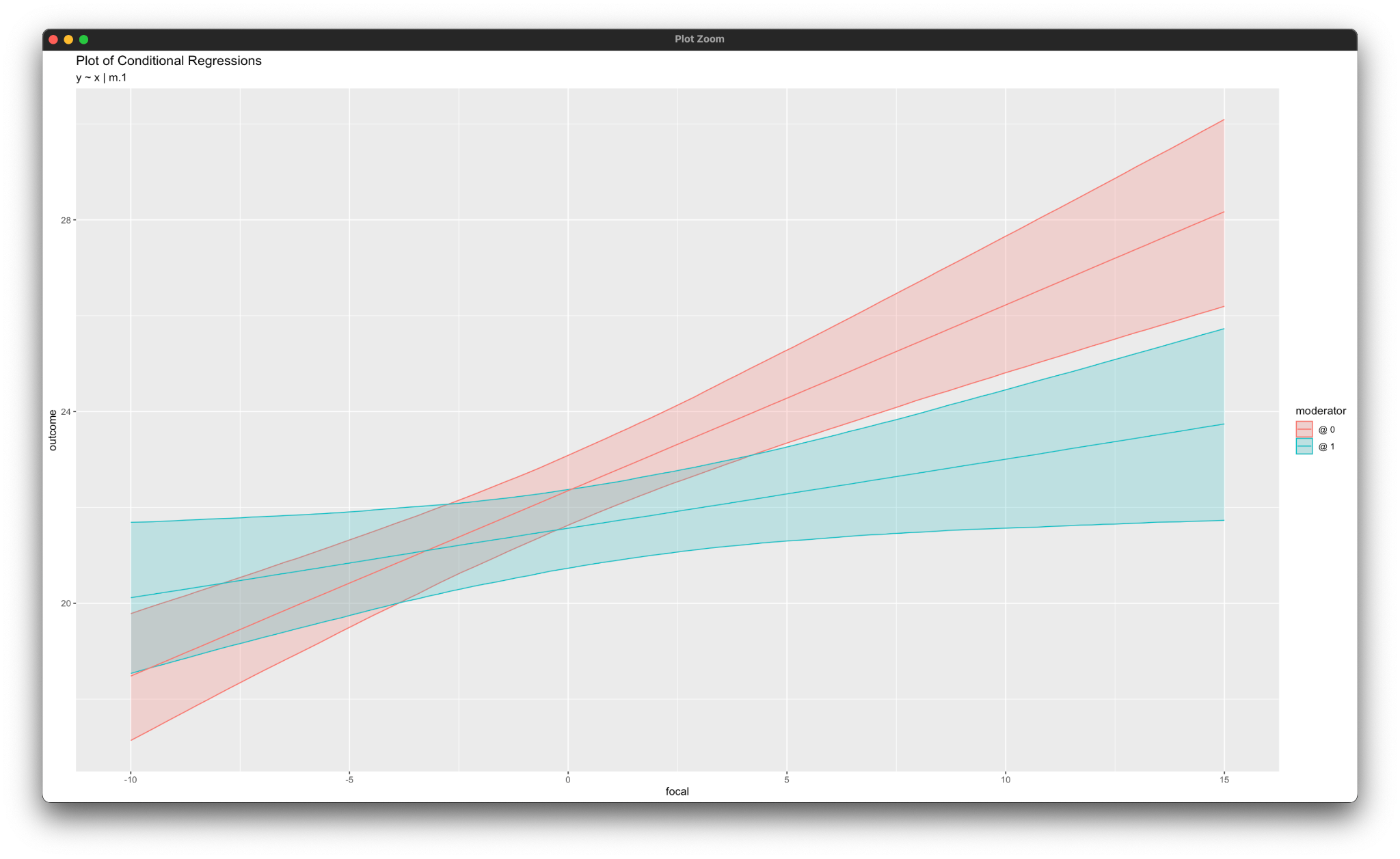
posterior_plot(mymodel)
simple_plot(y ~ x | m, mymodel)

The simple_plot function in the rblimp script produces graphs of simple intercepts and slopes. Note that, since the moderator m is defined as a nominal variable, the plotting function produces conditional regression slopes at each level of the moderator, as shown below. See the SIMPLE command in Section 2.20 for additional information.

Blimp can save multiple imputations from any model it estimates. The script below illustrates model-based multiple imputation (imputation tailored around one specific analysis) for the linear moderated regression model. The new syntax features are as follows.

CENTER command grand mean centers predictors in the Bayesian output, but saved imputations are on the original metric
NIMPS command specifies 20 imputed data sets (five data sets from each of the default four chains, sampled at equal intervals across the post-burn-in iterations)
Imputations are stacked in a single file with an index variable added in the first column

DATA: data4.dat;
VARIABLES: id v1:v3 y x v4 v5 d m v6:v24;
ORDINAL: d;
NOMINAL: m;
MISSING: 999;
FIXED: m;
CENTER: x;
MODEL: y ~ x m x*m d;
SIMPLE: x | m;
SEED: 90291;
BURN: 10000;
ITER: 10000;
NIMPS: 20;
SAVE: stacked = imps.dat;

VARIABLE ORDER IN IMPUTED DATA:

   stacked = 'imps.dat'

     imp# id a1 a2 a3 y x1 x2 n1 d1 d2 o1 o2 o3 o4 o5 o6 o7 o8
        o9 o10 o11 o12 o13 o14 o15 o16 o17 o18 o19

The imputed data sets can be analyzed in other software packages.

R provides an easy platform for analyzing multiple imputations. To illustrate, R script below uses rblimp to create multiple imputations and the mitml package (Grund, Robitzsch, & Lüdke, 2021) for analysis and pooling. Note that the SAVE command is no longer necessary because imputations are automatically stored in an rblimp list object called mymodel@imputations. The product term is not an imputed variable. Rather, the product is formed from the imputed lower-order variables, as shown below. The pooled multiple imputation estimates are numerically equivalent to the Bayesian results.

library(rblimp)

mymodel <- rblimp(
  data = data,
  ordinal = 'd',
  nominal = 'm',
  fixed = 'm',
  center = 'x',
  model = 'y ~ x m x*m d',
  simple = 'x | m',
  seed = 90291,
  burn = 10000,
  iter = 10000,
  nimps = 20
)

output(mymodel)
posterior_plot(mymodel)

# mitml list
implist <- as.mitml(mymodel)

# pooled grand mean
mean_x <- mean(unlist(lapply(implist, function(data) mean(data$x))))

# analysis and pooling with mitml
results <- with(implist, lm(y ~ I(x - mean_x) + m + I(x - mean_x):m + d))
testEstimates(results, extra.pars = T, df.com = 295)

4.9 Multiple Imputation Within Subgroups

Fully conditional specification multiple imputation is generally inappropriate for interactive effects because it is prone to bias. The moderated regression in Example 4.8 is an exception that could be handled by imputing the data separately within each group of the complete moderator variable (Enders & Gottschall, 2011; Graham, 2009). This example illustrates a multiple-group multiple imputation strategy that stratifies the data by subgroup and imputes within each strata.

The syntax highlights are as follows.

ORDINAL command identifies a binary variable
FIXED command identifies a complete variable
BYGROUP identifies complete, nominal strata variable not listed on the ORDINAL (or NOMINAL) command
FCS command includes all analysis variables (other than the one listed on the BYGROUP line) plus three auxiliary variables
NIMPS command specifies 20 imputed data sets (five data sets from each of the default four chains, sampled at equal intervals across the post-burn-in iterations)
Imputations are stacked in a single file with an index variable added in the first column

DATA: data4.dat;
VARIABLES: id a1:a3 y x v1 v2 d group v3:v21;
ORDINAL: d;
MISSING: 999;
FIXED: group;
BYGROUP: group;
FCS: a1:a3 y x d;
SEED: 90291;
BURN: 10000;
ITER: 10000;
NIMPS: 20;
SAVE: stacked = imps.dat;

VARIABLE ORDER IN IMPUTED DATA:

   stacked = 'imps.dat'

     imp# id a1 a2 a3 y x v1 v2 d group v3 v4 v5 v6 v7 v8 v9  
     v10 v11 v12 v13 v14 v15 v16 v17 v18 v19 v20 v21

The imputed data sets can be analyzed in other software packages.

library(rblimp)

mymodel <- rblimp_fcs(
  data = data,
  ordinal = 'd',
  variables = 'a1:a3 y x d',
  seed = 90291,
  burn = 10000,
  iter = 10000,
  nimps = 20
  ) |> by_group('group')

lapply(mymodel,output)

# mitml list
implist <- as.mitml(mymodel)

# pooled grand mean
mean_x <- mean(unlist(lapply(implist, function(data) mean(data$x))))

# analysis and pooling with mitml
results <- with(implist,
  lm(y ~ I(x - mean_x) + group + I(x - mean_x):group + d))
testEstimates(results, extra.pars = T, df.com = 295)

4.10 Curvilinear Regression

This example illustrates a curvilinear regression with a quadratic term and continuous and binary covariates. The regression model is as follows, and the c superscript denotes variables centered at their grand means.

\[y=\beta_0+\beta_1x_1^{c}+\beta_2(x_1^{c})^2+\beta_3x_2^{c}+\beta_4d_1+\beta_5d_2+\varepsilon\]

The syntax highlights are listed below.

ORDINAL command identifies binary predictors
FIXED command identifies complete predictors (optional—speeds computation)
CENTER command applies grand mean centering to predictors
MODEL command features an embedded function that squares a predictor
Unspecified associations for predictor variables

DATA: data5.dat;
VARIABLES: id d1 d2 v1:v3 x1 x2 y;
MISSING: 999;
ORDINAL: d1 d2;
FIXED: d1 x2;
CENTER: x1 x2;
MODEL: y ~ x1 (x1^2) x2 d1 d2;
SEED: 12345;
BURN: 10000;
ITER: 10000;

The corresponding rblimp script is as follows.

library(rblimp)

mymodel <- rblimp(
  data = data,
  ordinal = 'd1 d2',
  fixed = 'd1 x2',
  center = 'x1 x2',
  model = 'y ~ x1 (x1^2) x2 d1 d2',
  seed = 12345,
  burn = 10000,
  iter = 10000
)

output(mymodel)

4.11 Probit Regression With a Binary Outcome

This example illustrates probit regression for a binary outcome. The model features a latent response variable regressed on continuous predictors and a binary dummy code, and the c superscript denotes variables centered at their grand means.

\[y^\ast=\beta_0+\beta_1x_1^{c}+\beta_2x_2^{c}+\beta_3d+\varepsilon\]

A single threshold value fixed at zero is automatically included and does not require specification.

The syntax highlights are listed below.

ORDINAL command identifies a binary outcome and predictor
FIXED command identifies complete predictors (optional—speeds computation)
CENTER command applies grand mean centering to predictors
Unspecified associations for predictor variables

DATA: data1.dat;
VARIABLES: id v1 y v2 x1 x2 d v3 v4;
ORDINAL: y d;
MISSING: 999;
FIXED: d;
CENTER: x1 x2;
MODEL: y ~ x1 x2 d;
SEED: 90291;
BURN: 10000;
ITER: 10000;

The corresponding rblimp script is as follows.

library(rblimp)

mymodel <- rblimp(
  data = data,
  ordinal = 'y d',
  fixed = 'd',
  center = 'x1 x2',
  model = 'y ~ x1 x2 d',
  seed = 90291,
  burn = 10000,
  iter = 10000
)
output(mymodel)

Blimp can also create auxiliary parameters that are functions of the estimated model parameters. To illustrate, the following script uses parameter labels, built-in functions, and the PARAMETERS command to compute the predicted probability of a “success” or “case” at each level of the d dummy code (and at the means of the continuous predictors). The additional syntax highlights are as follows.

MODEL command labels the intercept and the binary predictor’s slope
PARAMETERS command defines news parameters that give the predicted probability of a “success” (outcome = 1) at each level of the dummy code and the group difference on the probability metric

DATA: data1.dat;
VARIABLES: id v1 y v2 x1 x2 d v3 v4;
ORDINAL: y d;
MISSING: 999;
FIXED: d;
CENTER: x1 x2;
MODEL: y ~ 1@b0 x1 x2 d@b3;
PARAMETERS:
  # conditional predicted probabilities
  pp_d0 = phi(b0);
  pp_d1 = phi(b0 + b3);
  pp_diff = pp_d1 - pp_d0;
SEED: 90291;
BURN: 10000;
ITER: 10000;

The corresponding rblimp script is shown below. In addition to creating predicted probabilities from the model parameters, the script below also saves multiply imputed estimates of the individual-level predicted probabilities. These imputations can be used to obtain marginal effects that average over the individual probabilities, as shown below using the mitml package.

library(rblimp)

mymodel <- rblimp(
  data = data,
  ordinal = 'y d',
  fixed = 'd',
  center = 'x1 x2',
  model = 'y ~ 1@b0 x1 x2 d@b3',
  parameters = '
    # conditional predicted probabilities
    pp_d0 = phi(b0);
    pp_d1 = phi(b0 + b3);
    pp_diff = pp_d1 - pp_d0',
  seed = 90291,
  burn = 10000,
  iter = 10000,
  nimps = 20
)

output(mymodel)
posterior_plot(mymodel, 'y')

# inspect variable names
names(mymodel@imputations[[1]])

# compare marginal predicted probabilities by group
implist <- as.mitml(mymodel)
results <- with(implist, lm(y.1.probability ~ 0 + d + I(1 - d)))
testEstimates(results)
confint.mitml.testEstimates(testEstimates(results))
testConstraints(results, constraints = c("d - `I(1 - d)`"))

4.12 Probit Regression With an Ordinal Outcome

This example illustrates a probit regression for an ordered categorical outcome with seven response options (e.g., a Likert scale). The model features a latent response variable regressed on continuous predictors and a binary dummy code, and the c superscript denotes variables centered at their grand means.

\[y^\ast=\beta_0+\beta_1x_1^{c}+\beta_2x_2^{c}+\beta_3d+\varepsilon\]

Six threshold parameters that divide the latent response distribution into seven bins are automatically included and do not require specification (the lowest is fixed at zero for identification).

The syntax highlights are listed below.

ORDINAL command identifies an ordinal outcome and a binary predictor
Automatic threshold specification for binary and ordinal variables
FIXED command identifies complete predictors (optional—speeds computation)
CENTER command applies grand mean centering to predictors
Unspecified associations for predictor variables
Longer burn-in period for ordered categorical variables

DATA: data1.dat;
VARIABLES: id v1 v2 y x1 x2 d v3 v4;
ORDINAL: y d;
MISSING: 999;
FIXED: d;
CENTER: x1 x2;
MODEL: y ~ x1 x2 d;
SEED: 90291;
BURN: 20000;
ITER: 20000;

The corresponding rblimp script is as follows.

library(rblimp)

mymodel <- rblimp(
  data = data,
  ordinal = 'y d',
  fixed = 'd',
  center = 'x1 x2',
  model = 'y ~ x1 x2 d',
  seed = 90291,
  burn = 20000,
  iter = 20000
)

output(mymodel)
posterior_plot(mymodel,'y')

4.13 Logistic Regression With a Binary Outcome

This example illustrates logistic regression for a binary outcome. The model features a binary outcome regressed on continuous predictors and a binary dummy code, and the c superscript denotes variables centered at their grand means.

\[\operatorname{ln}\left(\frac{Pr\left(y=1\right)}{1-Pr\left(y=1\right)}\right)=\beta_0+\beta_1x_1^{c}+\beta_2x_2^{c}+\beta_3d\]

The syntax highlights are listed below. When saving imputations, adding the savepredicted keyword to the OPTIONS command saves predicted probabilities (see Example 4.21).

ORDINAL command identifies a binary outcome and predictor
FIXED command identifies complete predictors (optional—speeds computation)
CENTER command applies grand mean centering to predictors
Applying the logit function to the dependent variable on the MODEL line requests a logit rather than probit link
Unspecified associations for predictor variables

DATA: data1.dat;
VARIABLES: id v1 y v2 x1 x2 d v3 v4;
ORDINAL: y d;
MISSING: 999;
FIXED: d;
CENTER: x1 x2;
MODEL: logit(y) ~ x1 x2 d;
SEED: 90291;
BURN: 10000;
ITER: 10000;

Note that the outcome variable must be coded as 0 and 1 when using the logit command in conjunction with ORDINAL. If the outcome has different codes (e.g., 1 and 2), either use TRANSFORM to recode the variable or use the NOMINAL command to identify the outcome as categorical, as follows.

DATA: data1.dat;
VARIABLES: id v1 y v2 x1 x2 d v3 v4;
ORDINAL: d;
NOMINAL: y;
MISSING: 999;
FIXED: d;
CENTER: x1 x2;
MODEL: y ~ x1 x2 d;
SEED: 90291;
BURN: 10000;
ITER: 10000;

The corresponding rblimp script is as follows.

library(rblimp)

mymodel <- rblimp(
  data = data,
  ordinal = 'y d',
  fixed = 'd',
  center = 'x1 x2',
  model = 'logit(y) ~ x1 x2 d',
  seed = 90291,
  burn = 10000,
  iter = 10000
)
output(mymodel)

The alternative specification using the NOMINAL command is as follows.

library(rblimp)

mymodel <- rblimp(
  data = data,
  ordinal = 'd',
  nominal = 'y',
  fixed = 'd',
  center = 'x1 x2',
  model = 'y ~ x1 x2 d',
  seed = 90291,
  burn = 10000,
  iter = 10000
)
output(mymodel)

MODEL command labels the intercept and the binary predictor’s slope
PARAMETERS command defines news parameters that give the predicted probability of a “success” (outcome = 1) at each level of the dummy code and the group difference on the probability metric

DATA: data1.dat;
VARIABLES: id v1 y v2 x1 x2 d v3 v4;
ORDINAL: y d;
MISSING: 999;
FIXED: d;
CENTER: x1 x2;
MODEL: logit(y) ~ 1@b0 x1 x2 d@b3;
PARAMETERS:
  # conditional predicted probabilities
  pp_d0 = exp(b0) / (1 + exp(b0));
  pp_d1 = exp(b0 + b3) / (1 + exp(b0 + b3));
  pp_diff = pp_d1 - pp_d0;
SEED: 90291;
BURN: 10000;
ITER: 10000;

The corresponding rblimp script is shown below. In addition to creating predicted probabilities from the model parameters, the script below also saves multiply imputed estimates of the individual predicted probabilities. These imputations can be used to obtain marginal effects that average over the individual probabilities, as shown below using the mitml package.

library(rblimp)
library(mitml)

mymodel <- rblimp(
  data = data,
  ordinal = 'y d',
  fixed = 'd',
  center = 'x1 x2',
  model = 'logit(y) ~ 1@b0 x1 x2 d@b3',
  parameters = '
    # conditional predicted probabilities
    pp_d0 = exp(b0) / (1 + exp(b0));
    pp_d1 = exp(b0 + b3) / (1 + exp(b0 + b3));
    pp_diff = pp_d1 - pp_d0',
  seed = 90291,
  burn = 10000,
  iter = 10000,
  nimps = 20
)

output(mymodel)
posterior_plot(mymodel, 'y')

# inspect variable names
names(mymodel)

# compare marginal predicted probabilities by group
implist <- as.mitml(mymodel)
results <- with(implist, lm(y.predicted ~ 0 + d + I(1 - d)))
testEstimates(results)
confint.mitml.testEstimates(testEstimates(results))
testConstraints(results, constraints = c("d - `I(1 - d)`"))

4.14 Logistic Regression With a Multicategorical Outcome

This example illustrates logistic regression for a multicategorical outcome with three levels. The model features a 3-category outcome (y = 1, 2, 3) regressed on three continuous predictors, with the lowest numeric code (e.g., y = 1) as the reference group. The c superscript denotes variables centered at their grand means.

\[\operatorname{ln}\left(\frac{Pr\left(y=2\right)}{Pr\left(y=1\right)}\right)=\beta_{02}+\beta_{12}x_1^{c}+\beta_{22}x_2^{c}+\beta_3x_3^{c}\]

\[\operatorname{ln}\left(\frac{Pr\left(y=3\right)}{Pr\left(y=1\right)}\right)=\beta_{03}+\beta_{13}x_1^{c}+\beta_{23}x_2^{c}+\beta_{33}x_3^{c}\]

The syntax highlights are listed below.

NOMINAL command identifies a multicategorical outcome, which automatically invokes a logit link when the categorical variable is an outcome (applying the logit function to the dependent variable is optional)
FIXED command identifies complete predictors (optional—speeds computation)
CENTER command applies grand mean centering to predictors
Unspecified associations for predictor variables

DATA: data4.dat;
VARIABLES: id x1:x3 v1:v3 y v4:v24;
NOMINAL: y;
MISSING: 999;
FIXED: x2 x3;
CENTER: x1 x2 x3;
MODEL: y ~ x1 x2 x3;
SEED: 90291;
BURN: 10000;
ITER: 10000;

The corresponding rblimp script is as follows.

library(rblimp)

mymodel <- rblimp(
  data = data,
  nominal = 'y',
  fixed = 'x2 x3',
  center = 'x1 x2 x3',
  model = 'y ~ x1 x2 x3',
  seed = 90291,
  burn = 10000,
  iter = 10000
)
output(mymodel)
posterior_plot(mymodel,'y')

4.15 Count Regression

This example illustrates a regression analysis with a count outcome. Blimp uses the negative binomial regression model described by Asparouhov and Muthén (2021). The negative binomial (NB) model is similar to the Poisson model, but it incorporates an additional overdispersion term that accounts for heterogeneity among individuals with the same predicted score. The interpretation of the coefficients is the same as a Poisson regression (Coxe, West, & Aiken, 2009). The model features a pair of continuous predictors and a binary dummy code, as follows. The c superscript denotes variables centered at their grand means.

\[\operatorname{ln}(\hat{\mu})=\beta_0+\beta_1d_1+\beta_2d_2+\beta_3x_1^{c}+\beta_4x_2^{c}\]

The term inside the natural log is the predicted count given the constellation of predictors on the right side of the equation. The model parameters reflect changes on the natural log of the count. As noted earlier, the model incorporates an overdispersion parameter that accommodates heterogeneity among individuals with the same predicted value.

The syntax highlights are as follows.

ORDINAL command identifies binary predictors
COUNT command identifies a count outcome
FIXED command identifies complete predictors (optional—speeds computation)
CENTERcommand applies grand mean centering to predictors
Unspecified associations for predictor variables

DATA: data22.dat;
VARIABLES: id d1 x1 v1 d2 x2 v2 y v3 v4;
ORDINAL: d1 d2;
COUNT: y;
MISSING: 999;
FIXED: d1 x1;
CENTER: x1 x2;
MODEL: y ~ d1 d2 x1 x2;
SEED: 90291;
BURN: 10000;
ITER: 10000;

The corresponding rblimp script is as follows.

library(rblimp)

mymodel <- rblimp(
  data = data,
  ordinal = 'd1 d2',
  count = 'y',
  fixed = 'd1 x1',
  center = 'x1 x2',
  model = 'y ~ d1 d2 x1 x2',
  seed = 90291,
  burn = 10000,
  iter = 10000
)

output(mymodel)
posterior_plot(mymodel,'y')

4.16 Zero-Inflated Count Outcome

This example illustrates a regression analysis with a count outcome that features excessive zeros. Blimp uses the negative binomial regression model described by Asparouhov and Muthén (2021). The negative binomial (NB) model is similar to the Poisson model, but it incorporates an additional overdispersion term that accounts for heterogeneity among individuals with the same predicted score. The interpretation of the coefficients is the same as a Poisson regression (Coxe, West, & Aiken, 2009).

A two-part model like that from Olsen and Schafer (2001) is used for the zero inflation. The two-part model features a binary indicator ybin that equals zero if the count variable y equals zero and one if y is greater than zero. The binary indicator is the dependent variable in a probit regression model predicting whether the count is non-zero. In probit regression, the binary indicator appears as a normally distributed latent response variable. In the model below, the latent response (denoted by an asterisk superscript) is regressed on a pair of binary dummy codes and continuous predictors.

\[y_{bin}^\ast=\beta_0+\beta_1d_1+\beta_2d_2+\beta_3x_1^{c}+\beta_4x_2^{c}+\varepsilon\]

The c superscript denotes centering at their grand mean. The probit model includes a single threshold value that is automatically fixed at zero for identification. The residual variance is similarly fixed at one.

The second part of the model considers only the non-zero counts. The outcome is a recoded version of y that is missing whenever y (or Ybin) equals zero. In the example below, the non-zero counts are regressed on a pair of binary dummy codes and continuous covariates.

\[\operatorname{ln}(\hat{\mu})=\beta_0+\beta_1d_1+\beta_2d_2+\beta_3x_1^{c}+\beta_4x_2^{c}\]

The c superscript again denotes grand mean centering. The term inside the natural log is the predicted count given the constellation of predictors on the right side of the equation. The model parameters reflect changes on the natural log of the count. As noted earlier, the model incorporates an overdispersion parameter that accommodates heterogeneity among individuals with the same predicted value.

The syntax highlights are listed below.

ORDINAL command identifies binary predictors and the binary outcome indicating whether the count was greater than zero
COUNT command identifies a count outcome
TRANSFORM command creates the variables for the two-part model
FIXED command identifies complete predictors (optional—speeds computation)
CENTERcommand applies grand mean centering to predictors
Unspecified associations for predictor variables

DATA: data22.dat;
VARIABLES: id d1 x1 v1 d2 x2 v2 ycnt v3 v4;
ORDINAL: d1 d2;
ORDINAL: d1 d2 ybin;
COUNT: y;
TRANSFORM:
  y = missing(ycnt == 0, ycnt);
  ybin = ifelse(ycnt == 0, 0, 1);
MISSING: 999;
FIXED: d1 x1;
CENTER: x1 x2;
MODEL:
  y ~ d1 d2 x1 x2;
  ybin ~ d1 d2 x1 x2;
SEED: 90291;
BURN: 10000;
ITER: 10000;

The corresponding rblimp script is as follows.

library(rblimp)

mymodel <- rblimp(
  data = data,
  ordinal = 'd1 d2 ybin',
  count = 'y',
  transform = '
    y = missing(ycnt == 0, ycnt);
    ybin = ifelse(ycnt == 0, 0, 1)',
  fixed = 'd1 x1',
  center = 'x1 x2',
  model = '
    y ~ d1 d2 x1 x2;
    ybin ~ d1 d2 x1 x2',
  seed = 90291,
  burn = 10000,
  iter = 10000
)

output(mymodel)
posterior_plot(mymodel)

4.17 Scale Scores With Incomplete Item Responses

This example illustrates a regression analysis that features a 6-item sum (scale) score as the outcome, a 7-item sum score as a predictor, and two binary covariates. The ordered categorical (e.g., questionnaire) items that determine the sum are incomplete. The analysis model is

\[y=\beta_0+\beta_1x+\beta_2d_1+\beta_3d_2+\varepsilon\]

\[=\beta_0+\beta_1\left(x_1+\ldots+x_7\right)+\beta_2d_1+\beta_3d_2+\varepsilon\]

where x is the scale (sum) score, and x1 to x7 are its ordinal components. It is important to treat missing data at the item level when analyzing incomplete composite scores, as doing so maximizes power and precision. This example illustrates the approach from Alacam, Du, Enders, and Keller (2023) and Enders (2022). It is important to reiterate that the scale score (represented as an embedded function) is essentially a random variable that depends on its constituent parts rather than a deterministic computation or passive imputation (see Section 2.19.11).

The syntax highlights are listed below.

ORDINAL command identifies binary and ordinal variables
Automatic threshold specification for binary and ordinal variables
MODEL command uses labels ending in a colon to group models and order their summary tables on the output
MODEL command features a syntax shortcut that creates a factored regression (sequential) specification for all predictors
MODEL command features an embedded function that defines the sum of ordinal items as a predictor
MODEL command defines the sum of ordinal items as a random variable

DATA: data4.dat;
VARIABLES: id v1:v3 yscale v4:v6 d1 d2
   y1:y6 x1:x7 v13:v18;
ORDINAL: x1:x7 d1 d2;
MISSING: 999;
MODEL:
  focal.model:
  xscale = x1:+:x7;         # definition variable for the sum score
    yscale ~  xscale d1 d2;   # embedded sum as a predictor
    predictor.model:
  x1:x7 d1 d2 ~ 1;
SEED: 90291;
BURN: 10000;
ITER: 10000;

The corresponding rblimp script is as follows.

library(rblimp)

mymodel <- rblimp(
  data = data,
  ordinal = 'x1:x7 d1 d2',
  model = '
    focal.model:
    xscale = x1:+:x7;          # definition variable for the sum score
      yscale ~  xscale d1 d2;    # embedded sum as a predictor
      predictor.model:
    x1:x7 d1 d2 ~ 1',
  seed = 90291,
  burn = 10000,
  iter = 10000
)

output(mymodel)
posterior_plot(mymodel,'yscale')

The previous script used a composite score as the dependent variable but did not incorporate the dependent variable’s component items into the model. Doing so would improve precision because the items are strong correlates of the sum score. The code block below leverages item-level correlations by introducing five of the six outcome items as auxiliary variables (Eekhout et al., 2015). The component items are added using the same auxiliary variable approach from Example 4.7. The additional syntax highlights are as follows.

MODEL command features a factored regression (sequential specification) for the dependent variable’s scale score and its items
All but one of the dependent variable’s scale items are used as auxiliary variables (using all items induces linear dependencies)

DATA: data4.dat;
VARIABLES: id a1 a2 a3 yscale v zscale n1 d1 d2
   y1:y6 x1:x7 z1:z6;
ORDINAL: x1:x7 d1 d2;
MISSING: 999;
MODEL:
  focal.model:
  xscale = x1:+:x7;
  yscale ~  xscale d1 d2;
  predictor.model:
  x1:x7 d1 d2 ~ 1;
  auxiliary.models:
  # sequential specification for y scale items
  y1:y5 ~ yscale;
SEED: 90291;
BURN: 20000;
ITER: 20000;

The corresponding rblimp script is as follows.

library(rblimp)

mymodel <- rblimp(
  data = data,
  ordinal = 'y1:y5 x1:x7 d1 d2',
  model = '
    focal.model:
    xscale = x1:+:x7;
    yscale ~  xscale d1 d2;
    predictor.model:
    x1:x7 d1 d2 ~ 1;
    auxiliary.models:
    y1:y5 ~ yscale',
  seed = 90291,
  burn = 20000,
  iter = 20000
)

output(mymodel)
posterior_plot(mymodel,'yscale')

4.18 Scale Score Interactions

This example illustrates a moderated regression with an interaction between a 7-item sum score predictor and binary moderator. The analysis model is

\[y=\beta_0+\beta_1x+\beta_2m+\beta_3(m)(x)+\varepsilon\]

\[=\beta_0+\beta_1\left(x_1+\ldots+x_7\right)+\beta_2m+\beta_3(m)\left(x_1+\ldots+x_7\right)+\varepsilon\]

where x is the scale (sum) score, and x1 to x7 are its ordinal components. It is important to treat missing data at the item level when analyzing incomplete composite scores, as doing so maximizes power and precision. This example extends the approach from Alacam, Du, Enders, and Keller (2023) to include interaction effects involving an incomplete sum score. Enders (2022) summarizes the approach. It is important to reiterate that the scale score (represented as an embedded function) is essentially a random variable that depends on its constituent parts rather than a deterministic computation or passive imputation (see Section 2.19.11).

The syntax highlights are listed below.

ORDINAL command identifies binary and ordinal variables
Automatic threshold specification for binary and ordinal variables
MODEL command uses labels ending in a colon to group models and order their summary tables on the output
MODEL command features a syntax shortcut that creates a factored regression (sequential) specification for all predictors
MODEL command features an embedded function that defines the sum of ordinal items as a predictor
MODEL command defines the sum of ordinal items as a random variable
MODEL command features a factored regression (sequential specification) for the dependent variable’s scale score and its items
All but one of the dependent variable’s scale items are used as auxiliary variables (using all items induces linear dependencies)
Longer burn-in period for estimating threshold parameters

DATA: data4.dat;
VARIABLES:
   id v1:v3 yscale zscale v4:v6 m
   y1:y6 x1:x7 v7:v12;
ORDINAL: y1:y5 x1:x7 m;
MISSING: 999;
MODEL:
  focal.model:
  xscale = x1:+:x7;
  yscale ~ xscale m m*xscale;
  predictor.model:
  x1:x7 m ~ 1;
  auxiliary.model:
  # sequential specification for y scale items
  y1:y5 ~ yscale;
SEED: 90291;
BURN: 20000;
ITER: 20000;

The corresponding rblimp script is as follows.

library(rblimp)

mymodel <- rblimp(
  data = data,
  ordinal = 'y1:y5 x1:x7 m',
  model = '
    focal.model:
    xscale = x1:+:x7;
    yscale ~ xscale m m*xscale;
    predictor.model:
    x1:x7 m ~ 1;
    auxiliary.model:
    y1:y5 ~ yscale',
  seed = 90291,
  burn = 20000,
  iter = 20000
)

output(mymodel)

4.19 Skewed Predictor With a Yeo–Johnson Transformation

This example illustrates a Yeo–Johnson (Yeo & Johnson, 2000) transformation that samples imputations from a skewed distribution. The analysis model is a logistic regression with two continuous variables and two binary dummy codes as predictors.

\[\operatorname{ln}\left(\frac{Pr\left(y=1\right)}{1-Pr\left(y=1\right)}\right)=\beta_0+\beta_1x_1+\beta_2x_2+\beta_3d_1+\beta_4d_2\]

x2’s distribution is markedly peaked and positively skewed, and drawing imputations from a normal distribution would likely distort the variable’s distribution.

The Yeo–Johnson procedure estimates the variableâs shape and draws imputations from a nonnormal distribution. Applying the Yeo–Johnson transformation normalizes the predictor variable, such that the resulting linear regression reflects associations between the normalized variable and other predictors. The sequential specification in the code block below invokes the following regression equation for the normalized predictor.

\[{\widetilde{x}}_2=\gamma_0+\gamma_1x_1+\gamma_2d_1+r\]

However, skewed imputations on the raw score metric always appear on the right side of any regression equation (e.g., the focal regression model). Normalized imputations can be saved by adding the savelatent keyword to the OPTIONS line.

The Yeo–Johnson transformation can be very slow (or fail) to converge if the skewed variable’s mean is far from zero. To facilitate interpretation, the code block below centers the predictor scores at the value of 15, which is roughly in the middle of the data. Additional details about the procedure are available in the literature (Enders, 2022; Lüdtke et al., 2020b).

The syntax highlights are listed below.

ORDINAL command identifies a binary outcome and predictors
FIXED command identifies complete predictors (optional—speeds computation)
MODEL command uses labels ending in a colon to group models and order their summary tables on the output
MODEL command features a factored regression (sequential specification) for incomplete predictor variables
Unspecified associations for complete predictor variables
Applying the yjt function to the skewed predictor on the MODEL line requests a Yeo–Johnson transformation
Applying a subtraction function to center the skewed predictor at its median facilitates convergence
Applying the logit function to the dependent variable on the MODEL line requests a logit rather than probit link

DATA: data6.dat;
VARIABLES: id d1 x1 v1 d2 v2 x2 v3 v4 y;
ORDINAL: y d1 d2;
MISSING: 999;
FIXED: d1 x1;
MODEL:
  focal.model:
  logit(y) ~ x1 x2 d1 d2;
  predictor.model:
  yjt(x2 - 15) ~ x1 d1;
  d2 ~ x2 x1 d1;
SEED: 90291;
BURN: 10000;
ITER: 10000;

The corresponding rblimp script is as follows.

library(rblimp)

mymodel <- rblimp(
  data = data,
  ordinal = 'y d1 d2',
  fixed = 'd1 x1',
  model = '
    focal.model:
    logit(y) ~ x1 x2 d1 d2;
    predictor.model:
    yjt(x2 - 15) ~ x1 d1;
    d2 ~ x2 x1 d1',
  seed = 90291,
  burn = 10000,
  iter = 10000
)

output(mymodel)
posterior_plot(mymodel)

4.20 Skewed Outcome With a Yeo–Johnson Transformation

This example applies the Yeo–Johnson transformation to a nonnormal dependent variable. The untransformed analysis model features two continuous variables and one binary dummy code as predictors, where the c superscript denotes variables centered at their grand means.

\[y=\beta_0+\beta_1x_1^{c}+\beta_2x_2^{c}+\beta_3d+\varepsilon\]

The outcome variableâs distribution is markedly peaked and positively skewed. Applying the Yeo–Johnson transformation normalizes the dependent variable, such that the resulting linear regression reflects associations between the normalized outcome and the predictors.

\[\widetilde{y}=\gamma_0+\gamma_1x_1^{c}+\gamma_2x_2^{c}+\gamma_3d+r\]

Normalized imputations can be saved by adding the savelatent keyword to the OPTIONS line. The Yeo–Johnson transformation can be very slow (or fail) to converge if the skewed variable’s mean is far from zero. To facilitate interpretation, the code block below centers the outcome at a value of 9, which is roughly in the middle of the data. Additional details about the procedure are available in the literature (Enders, 2022; Lüdtke et al., 2020b).

The syntax highlights are listed below.

ORDINAL command identifies a binary predictor
FIXED command identifies complete predictors (optional—speeds computation)
Applying yjt function to the skewed outcome on the MODEL line requests a Yeo–Johnson transformation
Applying a subtraction function to center the skewed outcome at its median facilitates convergence
Unspecified associations for predictor variables

DATA: data2.dat;
VARIABLES: id y v1 x1 d v2 v3 x2 v4;
ORDINAL: d;
MISSING: 999;
FIXED: x1;
CENTER: x1 x2;
MODEL: yjt(y - 9) ~ x1 x2 d;
SEED: 90291;
BURN: 10000;
ITER: 10000;

The corresponding rblimp script is as follows.

library(rblimp)

mymodel <- rblimp(
  data = data,
  ordinal = 'd',
  fixed = 'x1',
  center = 'x1 x2',
  model = 'yjt(y - 9) ~ x1 x2 d',
  seed = 90291,
  burn = 10000,
  iter = 10000
)

output(mymodel)
posterior_plot(mymodel)

Blimp can save multiple imputations from any model it estimates. When saving multiple imputations, listing the savelatent keyword on the OPTIONS command saves the normalized imputes from the Yeo–Johnson transformation alongside the skewed imputes on the raw score metric (this keyword also saves the latent response scores for the binary predictor).

DATA: data2.dat;
VARIABLES: id y n1 x1 d1 d2 n2 x2 n3;
ORDINAL: d1;
MISSING: 999;
FIXED: x1;
CENTER: x1 x2;
MODEL: yjt(y - 9) ~ x1 x2 d1;
SEED: 90291;
BURN: 10000;
ITER: 10000;
# save model-based multiple imputations;
NIMPS: 20;
OPTIONS: savelatent;
SAVE: stacked = imps.dat;

VARIABLE ORDER IN IMPUTED DATA:

   stacked = 'imps.dat'
     imp# id y v1 x1 d v2 v3 x2 v4 y.yjt d.latent

The variable y contains skewed imputations on the raw score metric, and the variable y.yjt contains the normalized imputes. The imputed data sets can be analyzed in other software packages.

To illustrate, the script below uses the R package mitml (Grund et al., 2021) to fit the regression model to the filled-in data sets. The positively skewed raw score imputations are on the original metric, whereas the transformed imputations are approximately normal.

# read data from working directory
imps <- read.table("imps.dat")
names(imps) <- c("imputation","id","y","v1","x1","d",
   "v2","v3","x2","v4","y.yjt","d1.latent")

# plot raw and transformed scores
hist(imps$y)
hist(imps$y.yjt)

# center predictors
imps$x1_cgm <- imps$x1 - mean(imps$x1)
imps$x2_cgm <- imps$x2 - mean(imps$x2)

# analysis and pooling with mitml
implist <- mitml::as.mitml.list(split(imps, imps$imputation))

# analyze skewed outcome
results <- with(implist, lm(y ~ x1_cgm  + x2_cgm + d))
mitml::testEstimates(results, extra.pars = T, df.com = 1996)

# analyze transformed outcome
results <- with(implist, lm(y.yjt ~ x1_cgm  + x2_cgm + d))
mitml::testEstimates(results, extra.pars = T, df.com = 1996)

The rblimp package provides an easy platform for analyzing multiple imputations. To illustrate, R script below uses rblimp to create multiple imputations and the mitml package (Grund, Robitzsch, & Lüdke, 2021) for analysis and pooling. Note that the SAVE command is no longer necessary because imputations are automatically stored in an rblimp list object called mymodel@imputations. The normalized variable has the suffix .yjt appended to the original variable’s name (e.g., y.yjt in this example).

library(rblimp)
library(mitml)

mymodel <- rblimp(
  data = data,
  ordinal = 'd',
  fixed = 'x1',
  center = 'x1 x2',
  model = 'yjt(y - 9) ~ x1 x2 d',
  seed = 90291,
  burn = 10000,
  iter = 10000,
  chains = 20,
  nimps = 20
)

output(mymodel)
posterior_plot(mymodel)

# inspect variable names
names(mymodel@imputations[[1]])

# mitml list
implist <- as.mitml(mymodel)

# plot raw and transformed scores
dat2plot <- do.call(rbind, implist)
hist(dat2plot$y,breaks = 20)
hist(dat2plot$y.yjt, breaks = 20)

# pooled grand means
mean_x1 <- mean(unlist(lapply(implist, function(data) mean(data$x1))))
mean_x2 <- mean(unlist(lapply(implist, function(data) mean(data$x2))))

# analyze skewed outcome
results <- with(implist,
   lm(y ~ I(x1 - mean_x1)  + I(x2 - mean_x2) + d))
testEstimates(results, extra.pars = T, df.com = 1996)

# analyze normalized outcome
results <- with(implist,
   lm(y.yjt ~ I(x1 - mean_x1)  + I(x2 - mean_x2) + d))
testEstimates(results, extra.pars = T, df.com = 1996)

4.21 Propensity Score Estimation With Missing Data

This example illustrates propensity score estimation with missing data. The focal model features a binary dummy code (the “treatment” indicator) predicting a continuous outcome.

\[y=\beta_0+\beta_1d+\varepsilon\]

The propensity score model features the treatment indicator regressed on potential confounder variables and their higher-order interaction terms.

\[\operatorname{ln}\left(\frac{Pr\left(d=1\right)}{1-Pr\left(d=1\right)}\right)=\gamma_0+\gamma_1x_1+\gamma_2x_2+\gamma_3x_3+\gamma_4x_4+\gamma_5x_1x_2+\gamma_6x_1x_3+\gamma_7x_1x_4+\gamma_8x_2x_3+\gamma_9x_2x_4+\gamma_{10}x_3x_4\]

Because the treatment indicator d consists of naturally occurring groups, this variable could be incomplete, which it is here. In this case, it is important for propensity score estimation to account for both models.

The syntax highlights are listed below.

ORDINAL command identifies a binary outcome and predictor
FIXED command identifies complete predictors (optional—speeds computation)
Applying the logit function to the dependent variable on the MODEL line requests a logit rather than probit link
CENTER command applies grand mean centering to predictors
MODEL command uses labels ending in a colon to group models and order their summary tables on the output
MODEL command features a product term
The savepredicted keyword on the OPTIONS line saves the predicted probabilities of treatment group membership, which are the propensity scores
Unspecified associations for predictor variables
NIMPS command specifies 20 imputed data sets (five data sets from each of the default four chains, sampled at equal intervals across the post-burn-in iterations)
Imputations are stacked in a single file with an index variable added in the first column

DATA: data4.dat;
VARIABLES: id x1:x4 y v1 v2 d v3:v22;
ORDINAL: d;
MISSING: 999;
FIXED: x2 x3;
MODEL:
  focal.model:
  y ~ d;
  propensity.model:
  logit(d) ~ x1 x2 x3 x4 x1*x2 x1*x3 x1*x4 x2*x3 x2*x4 x3*x4;
SEED: 90291;
BURN: 10000;
ITER: 10000;
OPTIONS: savepredicted;
NIMPS: 20;
SAVE: stacked = imps.dat;

VARIABLE ORDER IN IMPUTED DATA:

   stacked = 'imps.dat'

     imp# id x1 x2 x3 x4 y v1 v2 d v3 v4 v5 v6 v7 v8 v9 v10 
     v11 v12 v13 v14 v15 v16 v17 v18 v19 v20 v21 v22 
     y.predicted d.predicted

The variable d.predicted contains the propensity scores. Following earlier examples, imputed data sets from Blimp can be analyzed in other software packages.

The corresponding rblimp script is as follows. Note that the SAVE command is no longer necessary because imputations are automatically stored in a rblimp list object called mymodel@imputations. Predicted probabilities are automatically stored in a rblimp list object called mymodel@predicted.

library(rblimp)

mymodel <- rblimp(
  data = data,
  ordinal = 'd',
  fixed = 'x2 x3',
  model = '
    focal.model:
    y ~ d;
    propensity.model:
    logit(d) ~ x1 x2 x3 x4 x1*x2 x1*x3 x1*x4 x2*x3 x2*x4 x3*x4',
  seed = 90291,
  burn = 10000,
  iter = 10000,
  nimps = 20
)

output(mymodel)
posterior_plot(mymodel)

4.22 Sampling Weights

This example illustrates a linear regression analysis with sampling (i.e., inverse probability) weights. The analysis model features three continuous predictors.

\[y=\beta_0+\beta_1x_1+\beta_2x_2+\beta_3x_3+\varepsilon\]

Blimp’s MCMC estimation routine incorporates sampling weights using the procedure described in Goldstein (2011, Section 3.4.2).

The syntax highlights are as follows.

WEIGHT command identifies the inverse probability sampling weights
Unspecified associations for predictor variables

DATA: data21.dat;
VARIABLES: v1:v3 wght y x1:x3 v4 v5;
WEIGHT: wght;
MISSING: 999;
MODEL: y ~ x1 x2 x3;
SEED: 90291;
BURN: 10000;
ITER: 10000;

The corresponding rblimp script is as follows.

library(rblimp)

mymodel <- rblimp(
  data = data,
  model = 'y ~ x1 x2 x3',
  weights = 'wght',
  seed = 90291,
  burn = 10000,
  iter = 10000
)

output(mymodel)
posterior_plot(mymodel)

4.23 Wald Significance Tests

This example illustrates the linear regression analysis from Example 4.3 with the Bayesian Wald test described by Asparouhov and Muthén (2021). These tests are printed by default for selected individual parameters. This example illustrates how to specify a custom significance test for evaluating the omnibus null hypothesis that all regression slopes equal zero. Other tests are possible as well (e.g., tests of equality constraints, nested model tests). The model features a pair of continuous predictors and a binary dummy code, where the c superscript denotes variables centered at their grand means.

\[y=\beta_0+\beta_1x_1^{c}+\beta_2x_2^{c}+\beta_3d+\varepsilon\]

The syntax highlights are as follows.

ORDINAL command identifies a binary predictor
FIXED command identifies complete predictors (optional—speeds computation)
CENTER command applies grand mean centering to predictors
WALDTEST commands specify three custom Bayesian Wald significance tests
Unspecified associations for predictor variables

DATA: data1.dat;
VARIABLES: id v1:v3 y x1 d x2 v4;
ORDINAL: d;
MISSING: 999;
FIXED: d;
CENTER: x1 x2;
MODEL: y ~ x1@b1 x2@b2 d@b3;
WALDTEST: b1:b3 = 0;
WALDTEST: b1:b2 = 0;
WALDTEST: b1 = b2;
SEED: 90291;
BURN: 10000;
ITER: 10000;

The corresponding rblimp script is as follows. Notice that each test is an element in a list.

library(rblimp)

mymodel <- rblimp(
  data = data,
  ordinal = 'd',
  fixed = 'd',
  center = 'x1 x2',
  model = 'y ~ x1@b1 x2@b2 d@b3',
  waldtest = list('b1:b3 = 0', 'b1:b2 = 0', 'b1 = b2'),
  seed = 90291,
  burn = 10000,
  iter = 10000)

output(mymodel)
posterior_plot(mymodel)

The WALDTESTcommand produces the output table below. The Wald test statistic is a chi-square variable, and the test’s degrees of freedom equals the number of parameters by which the two models differ. The chi-square is an MCMC-generated estimate of a frequentist test statistic, and the p-value is the area above the test statistic value in a chi-square distribution. As such, the test can be used for frequentist inference. This approach adopts MCMC estimation for its computational benefits rather than its philosophical appeal (i.e., Bayes as computational frequentism; Levy & McNeish, 2023). By default, Blimp prints univariate Wald tests for all parameters except variances and variance explained test statistics.

WALD TESTS (Asparouhov & Muthén, 2021)

  Test #1

    Full:
      [1]  y ~ Intercept x1@b1 x2@b2 d@b3

    Restricted:
      [1]  y ~ Intercept x1@b1 x2@b2 d@b3

    Constraints in Restricted:
      [1]  b1 = 0
      [2]  b2 = 0
      [3]  b3 = 0

    Wald Statistic (Chi-Square)               158.084
    Number of Parameters Tested (df)                3
    Probability                                 0.000

  Test #2

    Full:
      [1]  y ~ Intercept x1@b1 x2@b2 d@b3

    Restricted:
      [1]  y ~ Intercept x1@b1 x2@b2 d@b3

    Constraints in Restricted:
      [1]  b1 = 0
      [2]  b2 = 0

    Wald Statistic (Chi-Square)               113.818
    Number of Parameters Tested (df)                2
    Probability                                 0.000

  Test #3

    Full:
      [1]  y ~ Intercept x1@b1 x2@b2 d@b3

    Restricted:
      [1]  y ~ Intercept x1@b1 x2@b2 d@b3

    Constraints in Restricted:
      [1]  b1 = b2

    Wald Statistic (Chi-Square)                28.673
    Number of Parameters Tested (df)                1
    Probability                                 0.000