5 Path Analysis and Latent Variable Model Examples

This section illustrates path analyses and latent variable models in Blimp. These multivariate analyses are specified as collections of univariate equations. In general, it is possible to mix and match features from any examples to easily create complex analysis models that honor features of the data. Additional details about fitting path and latent variable models in Blimp can be found in Keller (2022), which is available for download here.

Following the previous chapter, the examples in this section use a generic notation system where variable names usually consist of an alphanumeric prefix and a numeric suffix (e.g., y, x1, x2, n1, d1, d2). The letter y designates a dependent variable, a d prefix denotes a binary dummy variable, an o prefix indicates an ordinal variable, and an n prefix indicates a multicategorical nominal variable. Finally, the model equations use a “c” superscript to indicate grand mean centering. The following list outlines the examples in this section.

5.1: Mediation Analysis
5.2: Moderated Mediation
5.3: Mediation With a Binary Outcome
5.4: Mediation With a Categorical Mediator
5.5: Mediation With a Count Outcome
5.6: Mediation With a Zero-Inflated Count Outcome
5.7: CFA With Continuous Indicators
5.8: CFA With Binary Indicators (2-Parameter IRT Model)
5.9: CFA With Ordinal Indicators
5.10: Imputing Latent Response Scores for Item-Level Factor Analysis
5.11: Skewed Indicators With a Yeo–Johnson Transformation
5.12: Latent Variable Regression Model
5.13: Latent-by-Manifest Variable Interaction
5.14: Moderated Nonlinear Factor Analysis (MNLFA)
5.15: Latent-by-Latent Variable Interaction
5.16: Three-Way Latent Variable Interaction
5.17: Latent Growth Curve Model
5.18: Residual SEM: AR1 Growth Model
5.19: Random Intercept Cross-Lagged Panel Model (RI-CLPM)

5.1 Mediation Analysis

This example illustrates a single-mediator path model. The regression models are shown below

\[m=I_m+{\alpha}x+\varepsilon_m\]

\[y=I_y+{\beta}m+{\tau}^{'}x+\varepsilon_y\]

where α and β are slope coefficients that define the indirect effect or product of the coefficients estimator, and τ’ is the direct effect of x on y. A path diagram of the analysis is shown below.

The full set of User Guide examples is available from the Examples pull-down menu in the Blimp Studio graphical interface. A GitHub repository with Blimp Studio scripts and data is available here, and a repository containing the rblimp scripts is available here.

The syntax highlights are as follows.

MODEL command uses labels ending in a colon to group models and order their summary tables on the output
MODEL command labels the indirect effect’s component pathways
PARAMETERS command uses labeled quantities to compute the product of coefficients estimator

DATA: data4.dat;
VARIABLES: id a1:a3 v1 y m v2 x v3:v22;
MISSING: 999;
MODEL:
  m ~ x@alpha;
  y ~ m@beta x;
PARAMETERS:
  indirect = alpha * beta;
SEED: 90291;
BURN: 10000;
ITER: 10000;

The corresponding rblimp script is as follows.

library(rblimp)

mymodel <- rblimp(
  data = data,
  model = '
    m ~ x@alpha;
    y ~ m@beta x;',
  parameters = 'indirect = alpha * beta',
  seed = 90291,
  burn = 10000,
  iter = 10000
)

output(mymodel)
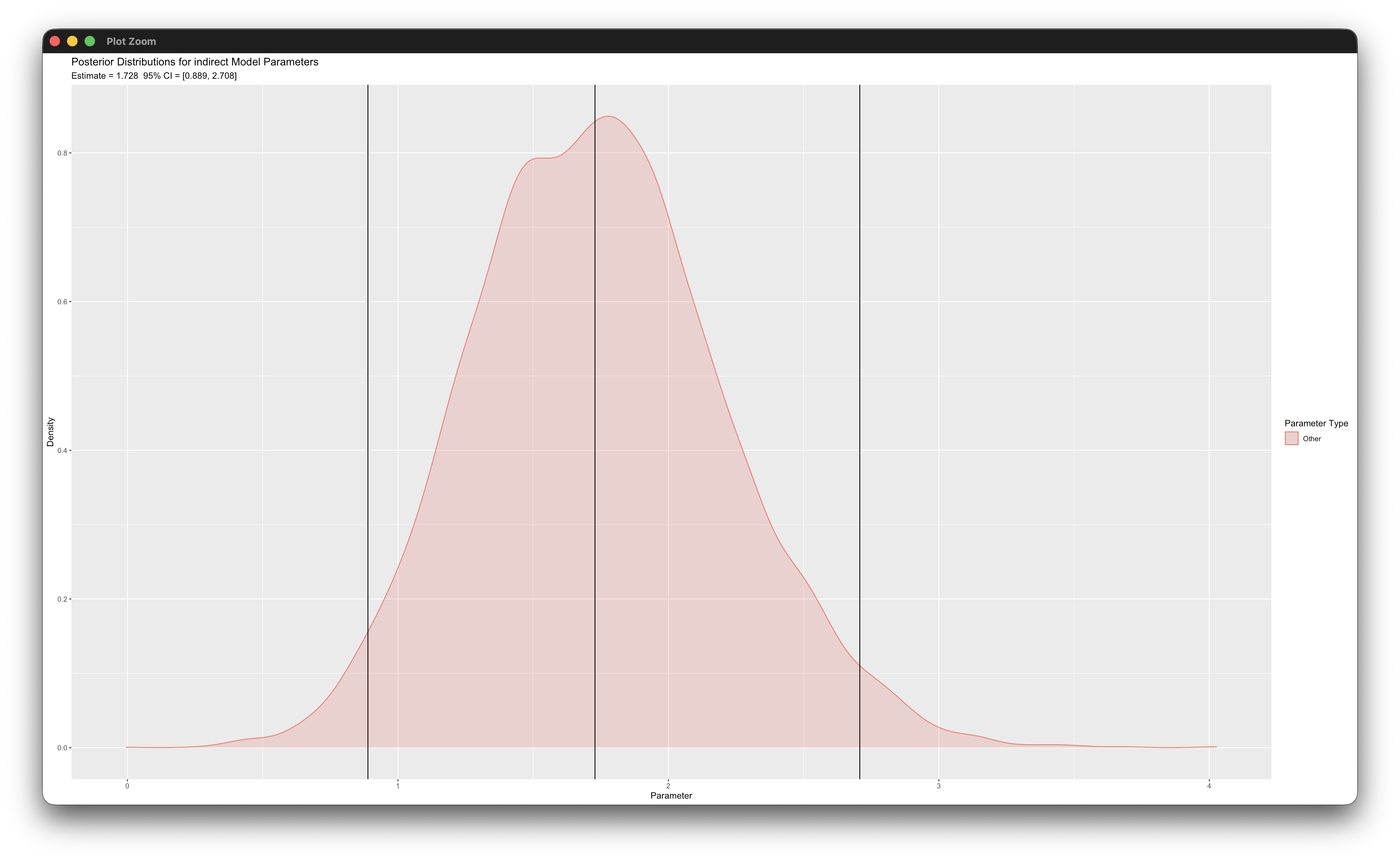
posterior_plot(mymodel,'indirect')
posterior_plot(mymodel)

Working in rblimp is advantageous because graphing functions are available for visualizing results. For example, the first posterior_plot function call graphs the distribution of the mediated effect, which is named indirect. The 95% intervals are asymmetric because the distribution is skewed, and the graph indicates that the indirect effect is significant because zero is not within the interval.

5.2 Moderated Mediation

This example adds moderated pathways to the single-mediator model from the previous example. The regression models are shown below

\[m=I_m+\alpha x+\gamma_1d+\gamma_2(x)(d)+\varepsilon_m\]

\[y=I_y + \beta m+\tau^{'}x+\gamma_3d+\gamma_4(m)( d)+\varepsilon_y\]

and the corresponding path diagram is as follows.

The dashed lines pointing from d to the directed arrows convey that d moderates the mediation model paths.

The syntax highlights are as follows.

ORDINAL command identifies a binary predictor
FIXED command identifies complete predictors (optional—speeds computation)
MODEL command uses labels ending in a colon to group models and order their summary tables on the output
MODEL command labels the indirect effect’s component pathways
MODEL command features a product term
PARAMETERS command uses labeled quantities to compute the product of coefficients estimator at each level of the binary moderator

DATA: data4.dat;
VARIABLES: id a1:a3 v1 y m v2 x d v3:v21;
ORDINAL: d;
MISSING: 999;
FIXED: d;
MODEL:
  m ~ x@alpha d x*d@alphadif;
  y ~ m@beta x d m*d@betadif;
PARAMETERS:
  indirect_d0 = alpha * beta;
  indirect_d1 = ( alpha + alphadif ) * ( beta + betadif );
  indirect_dif = indirect_d1 - indirect_d0;
SEED: 90291;
BURN: 10000;
ITER: 10000;

The corresponding rblimp script is as follows.

library(rblimp)

mymodel <- rblimp(
  data = data,
  ordinal = 'd',
  fixed = 'd',
  model = '
    m ~ x@alpha d x*d@alphadif;
    y ~ m@beta x d m*d@betadif;',
  parameters = '
    indirect_d0 = alpha * beta;
    indirect_d1 = ( alpha + alphadif ) * ( beta + betadif );
    indirect_dif = indirect_d1 - indirect_d0;',
  seed = 90291,
  burn = 10000,
  iter = 10000
)

output(mymodel)
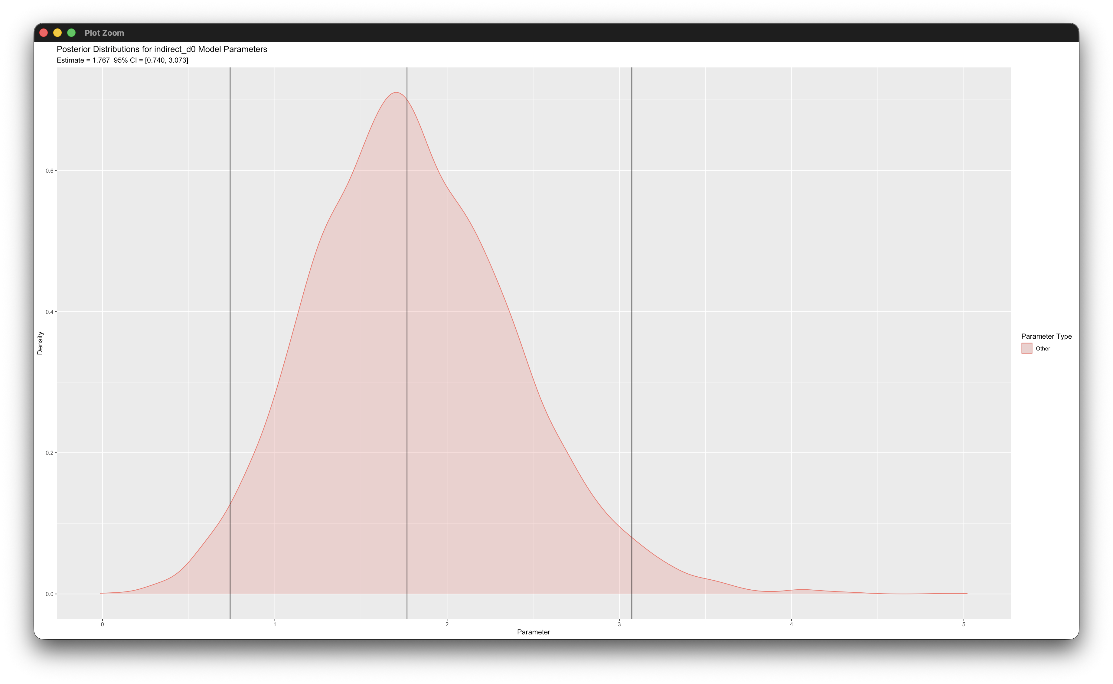
posterior_plot(mymodel,'indirect_d0')
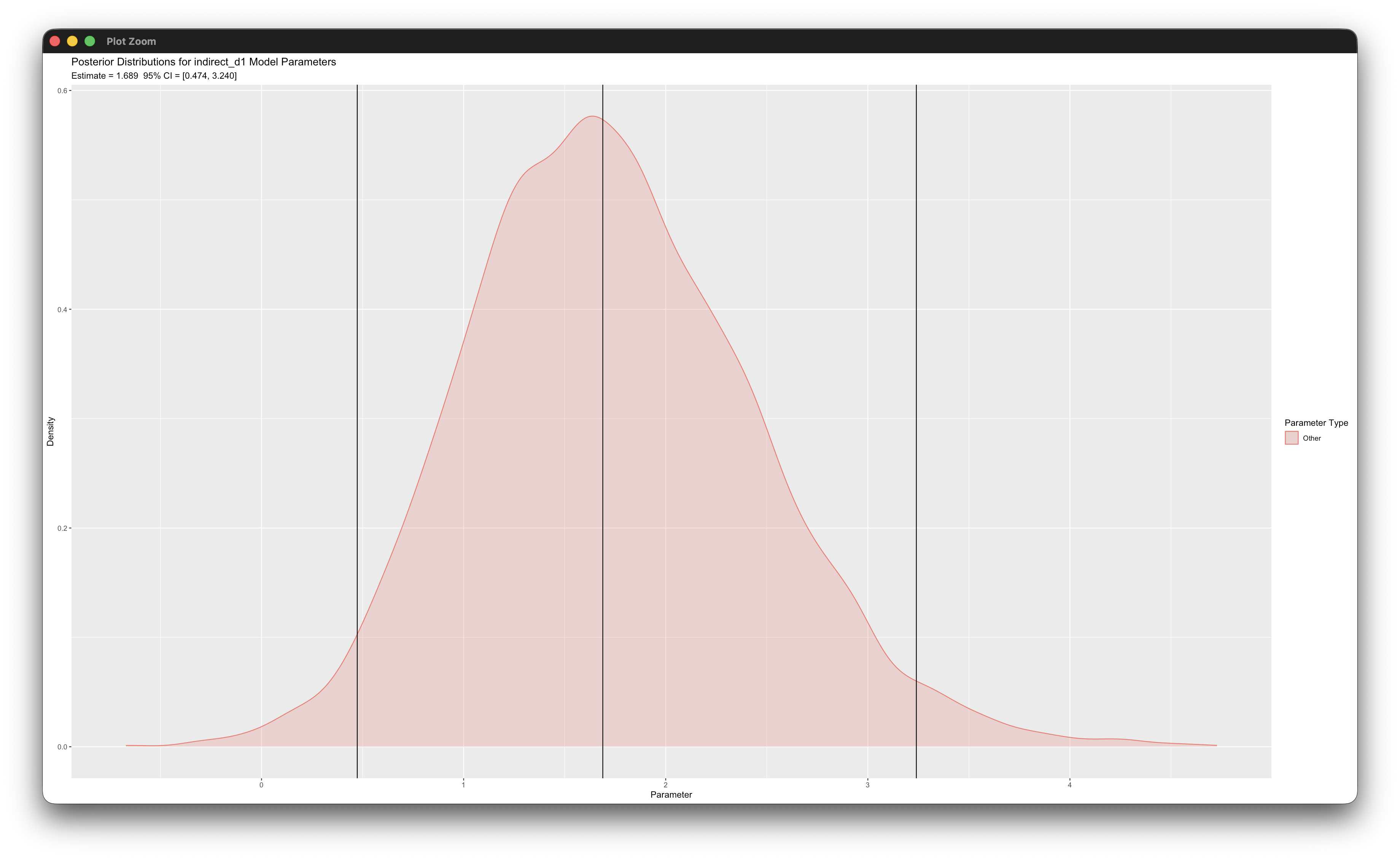
posterior_plot(mymodel,'indirect_d1')
posterior_plot(mymodel)

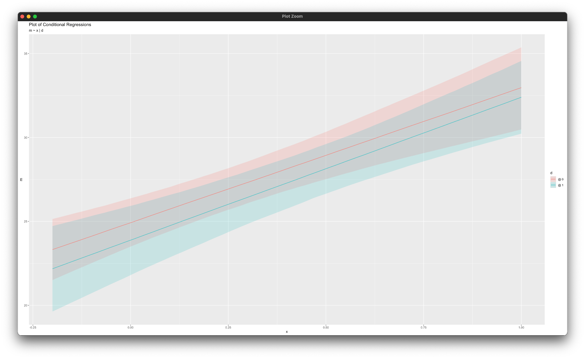
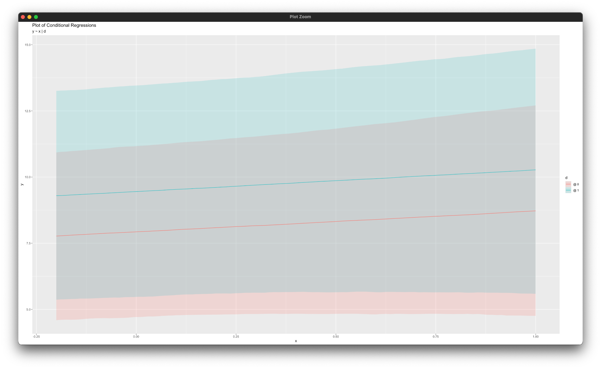
simple_plot(m ~ x | d, mymodel)
simple_plot(y ~ m | d, mymodel)

Working in rblimp is advantageous because graphing functions are available for visualizing results. For example, the first two posterior_plot function calls graph the distributions of the mediated effects, which are named indirect_d0 and indirect_d1. The 95% intervals are asymmetric because the distribution are skewed, and the graphs indicate that the indirect effects are significant because zero is not within the intervals.

Similarly, the simple_plot function calls produce graphs of simple intercepts and slopes for each mediated pathway, as shown below.

5.3 Mediation With a Binary Outcome

This example illustrates a single-mediator model with a binary outcome. The regression models are shown below

\[m=I_m+{\alpha}x+\varepsilon_m\]

\[y^{*}=I_y+{\beta}m+{\tau}^{'}x+\varepsilon_{y^*}\]

where y* denotes the underlying latent response variable for a binary outcome y, and all other features of the model are the same as Example 5.1. A path diagram of the mediation model is shown below, with the ellipse denoting the latent response variable, the residual variance of which is fixed at one for identification.

Muthén, Muthén, and Asparouhov (2016) show that the indirect effect alone does not capture the fact that changes in y are non-constant on the probability metric. They give the following expression for computing the probability that y = 1 given a particular value of x (Equations 8.4 to 8.6). The script below uses these equations to compute the probability at different values of x. These probabilities are the building blocks of their causally-defined indirect effect estimates in the examples below (the natural indirect effect, the natural direct effect, and the total effect).

\[E(y^*|x)=I_y+I_m{\beta}+{\alpha}{\beta}x+{\tau}^{'}x\] \[V(y^*|x)=\beta^2\sigma_m^2+1\]

\[P(y=1|x) = \phi[E(y^*|x)/\sqrt{V(y^*|x)}]\]

The syntax highlights are as follows.

ORDINAL command identifies a binary outcome and predictor
Unspecified associations for predictor variables
MODEL command uses labels ending in a colon to group models and order their summary tables on the output
MODEL command labels intercepts, slopes, and the residual variance of the mediator
PARAMETERS command uses labeled quantities to compute causally-defined indirect effect estimates

DATA: data20.dat;
VARIABLES: id a1:a3 v1 y m v2 x v3:v22;
MISSING: 999;
ORDINAL: x y;
MODEL:
  m ~ 1@m_icept x@alpha;
  m@m_resvar;
  y ~ 1@y_icept m@beta x@tau;
PARAMETERS:
  den = sqrt(beta^2*m_resvar + 1);
  # model-implied marginal probabilities at X=0 and X=1
  p_x0 = phi( ( y_icept + beta*(m_icept + alpha*0) + tau*0 ) / den );
  p_x1 = phi( ( y_icept + beta*(m_icept + alpha*1) + tau*1 ) / den );
  # natural Indirect Effect: P(Y=1 | X=1, M_{X=1}) - P(Y=1 | X=1, M_{X=0})
  nie = phi( ( y_icept + beta*(m_icept + alpha*1) + tau*1 ) / den )
    - phi( ( y_icept + beta*(m_icept + alpha*0) + tau*1 ) / den );
  # natural Direct Effect: P(Y=1 | X=1, M_{X=0}) - P(Y=1 | X=0, M_{X=0})
  nde = phi( ( y_icept + beta*(m_icept + alpha*0) + tau*1 ) / den )
    - phi( ( y_icept + beta*(m_icept + alpha*0) + tau*0 ) / den );
  # total effect = P(Y=1|X=1) - P(Y=1|X=0) = NIE + NDE
  te  = p_x1 - p_x0;
SEED: 90291;
BURN: 10000;
ITER: 10000;

The corresponding rblimp script is as follows.

library(rblimp)

mymodel <- rblimp(
  data = data,
  ordinal = 'x y',
  model = '
    m ~ 1@m_icept x@alpha;
    m@m_resvar;
    y ~ 1@y_icept m@beta x@tau;',
  parameters = '
    den = sqrt(beta^2*m_resvar + 1);
    # model-implied marginal probabilities at X=0 and X=1
    p_x0 = phi( ( y_icept + beta*(m_icept + alpha*0) + tau*0 ) / den );
    p_x1 = phi( ( y_icept + beta*(m_icept + alpha*1) + tau*1 ) / den );
    # natural Indirect Effect: P(Y=1 | X=1, M_{X=1}) - P(Y=1 | X=1, M_{X=0})
    nie = phi( ( y_icept + beta*(m_icept + alpha*1) + tau*1 ) / den )
      - phi( ( y_icept + beta*(m_icept + alpha*0) + tau*1 ) / den );
    # natural Direct Effect: P(Y=1 | X=1, M_{X=0}) - P(Y=1 | X=0, M_{X=0})
    nde = phi( ( y_icept + beta*(m_icept + alpha*0) + tau*1 ) / den )
      - phi( ( y_icept + beta*(m_icept + alpha*0) + tau*0 ) / den );
    # total Effect = P(Y=1|X=1) - P(Y=1|X=0) = NIE + NDE
    te  = p_x1 - p_x0;',
  seed = 90291,
  burn = 10000,
  iter = 10000
)

output(mymodel)
posterior_plot(mymodel,'nie')
posterior_plot(mymodel,'nde')
posterior_plot(mymodel,'te')

The script above defines the binary outcome as a latent response variable (i.e., probit regression). Applying the logit function to the dependent variable on the MODEL line requests a logit rather than probit link.

\[m=I_m+{\alpha}x+\varepsilon_m\]

\[\operatorname{logit}(y)=I_y+{\beta}m+{\tau}^{'}x\]

The conditional probabilities from Muthén, Muthén, and Asparouhov (2016) shown above do not have a simple expression when using a logit link. Instead, we can use the conditional indirect effects expressions defined in Geldhof et al. (2018, p. 304). They define the conditional indirect effect at a given value of x as follows

\[\alpha\beta{ | } x =\alpha \times \frac{\beta \times e^{I_y + \beta m + {\tau}^{'}x}}{(1 + e^{I_y + \beta m + {\tau}^{'}x})^2}\]

The PARAMETERS command in the script below computes these conditional indirect effects at three values of x.

DATA: data20.dat;
VARIABLES: id a1:a3 v1 y m v2 x v3:v22;
MISSING: 999;
ORDINAL: x y;
MODEL:
  # single-mediator model with parameter labels
  m ~ 1@m_icept x@alpha;
  logit(y) ~ 1@y_icept m@beta x@tau;
PARAMETERS:
  # conditional indirect effect at X = 0
  ab_x0 = alpha * ( beta * exp( y_icept + beta*(m_icept + alpha*0) + tau*0 ) ) /
    ( 1 + exp( y_icept + beta*(m_icept + alpha*0) + tau*0 ) )^2;
  # conditional indirect effect at X = 1
  ab_x1 = alpha * ( beta * exp( y_icept + beta*(m_icept + alpha*1) + tau*1 ) ) /
    ( 1 + exp( y_icept + beta*(m_icept + alpha*1) + tau*1 ) )^2;
  # contrast
  ab_diff = ab_x1 - ab_x0;
SEED: 90291;
BURN: 10000;
ITER: 10000;

The corresponding rblimp script is as follows.

library(rblimp)

mymodel <- rblimp(
  data = data,
  ordinal = 'x y',
  model = '
    m ~ 1@m_icept x@alpha;
    logit(y) ~ 1@y_icept m@beta x@tau;',
  parameters = '
    # conditional indirect effect at X = 0
    ab_x0 = alpha * ( beta * exp( y_icept + beta*(m_icept + alpha*0) + tau*0 ) ) /
      ( 1 + exp( y_icept + beta*(m_icept + alpha*0) + tau*0 ) )^2;
    # conditional indirect effect at X = 1
    ab_x1 = alpha * ( beta * exp( y_icept + beta*(m_icept + alpha*1) + tau*1 ) ) /
      ( 1 + exp( y_icept + beta*(m_icept + alpha*1) + tau*1 ) )^2;
    # contrast
    ab_diff = ab_x1 - ab_x0;',
  seed = 90291,
  burn = 10000,
  iter = 10000
)

output(mymodel)
posterior_plot(mymodel,'ab_x0')
posterior_plot(mymodel,'ab_x1')
posterior_plot(mymodel,'ab_diff')
posterior_plot(mymodel)

5.4 Mediation With a Categorical Mediator

This example illustrates a single-mediator path model with an ordered categorical mediator (the mediator could also be binary). The regression models are shown below

\[m^{*}=I_m+{\alpha}x+\varepsilon_m^{*}\]

\[y=I_y+{\beta}m^{*}+{\tau}^{'}x+\varepsilon_y\]

When m is binary or ordinal, the 𝛼 path represents the regression of a latent response variable on x. Typically, the discrete m would then serve as a predictor of y, thus leading to an awkward situation where m essentially has two different metrics within the same model (i.e., m is latent when it is an outcome variable but ordinal when it is a predictor). Alternatively, Blimp can use the latent response variable in both regressions, effectively converting a complicated categorical variable regression into a straightforward linear regression with latent response variables. This idea was proposed in Muthén, Muthén, and Asparouhov (2016).

The syntax highlights are as follows.

ORDINAL command identifies an ordinal mediator
CENTER command applies grand mean centering to predictors
MODEL command uses labels ending in a colon to group models and order their summary tables on the output
MODEL command labels the indirect effect’s component pathways
Appending the .latent suffix to the mediator’s variable name in the MODEL statement accesses the latent response variable instead of the discrete responses
PARAMETERS command uses labeled quantities to compute the product of coefficients estimator

DATA: data4.dat;
VARIABLES: id a1:a3 v1 y v2 v3 x v4:v22 m;
MISSING: 999;
ORDINAL: m;
MODEL:
  m ~ x@alpha;
  y ~ m.latent@beta x;
PARAMETERS:
  indirect = alpha * beta;
SEED: 90291;
BURN: 10000;
ITER: 10000;

The corresponding rblimp script is as follows.

library(rblimp)

mymodel <- rblimp(
  data = data,
  ordinal = 'm',
  center = 'x',
  model = '
    m ~ x@alpha;
    y ~ m.latent@beta x;',
  parameters = 'indirect = alpha * beta',
  seed = 90291,
  burn = 10000,
  iter = 10000
)

output(mymodel)
posterior_plot(mymodel,'indirect')
posterior_plot(mymodel)

An alternate approach uses the conditional indirect effects expressions defined in Geldhof et al. (2018, p. 304). To illustrate, suppose that m is a binary mediator. The mediation model equations adopt a logistic model for m.

\[\operatorname{logit}(m)=I_m+{\alpha}x\]

\[y=I_y+\beta m+\tau^{'}x+\varepsilon_y\]

Applying the logit function to the mediator variable on the MODEL line requests a logit link for this variable. Geldhof et al. define conditional indirect effects that reflect changes to m on the probability metric as follows.

\[\alpha\beta{ | } x =\frac{\alpha \times e^{I_m + \alpha x}}{(1 + e^{I_m + \alpha x})^2} \times \beta\]

The PARAMETERS command in the script below computes these conditional indirect effects at three values of x.

DATA: data5.4b.dat;
VARIABLES: id a1:a3 v1 y v2 v3 x v4:v22 m;
MISSING: 999;
ORDINAL: m;
CENTER: x;
MODEL:
  logit(m) ~ 1@m_icept x@alpha;
  y ~ m@beta x;
PARAMETERS:
  xvalue1 = -.50;
  xvalue2 = 0;
  xvalue3 = .50;
  ab_xval1 = (alpha*exp(m_icept + alpha*xvalue1)) /
    (1 + exp(m_icept + alpha*xvalue1))^2 * beta;
  ab_xval2 = (alpha*exp(m_icept + alpha*xvalue2)) /
    (1 + exp(m_icept + alpha*xvalue2))^2 * beta;
  ab_xval3 = (alpha*exp(m_icept + alpha*xvalue3)) /
    (1 + exp(m_icept + alpha*xvalue3))^2 * beta;
SEED: 90291;
BURN: 10000;
ITER: 10000;

The corresponding rblimp script is as follows.

library(rblimp)

mymodel <- rblimp(
  data = data,
  ordinal = 'm',
  transform = 'm = ifelse(m7pt <= 4, 0, 1)',
  center = 'x',
  model = '
    logit(m) ~ 1@m_icept x@alpha;
    y ~ m@beta x;',
  parameters = '
    xvalue1 = -.50;
    xvalue2 = 0;
    xvalue3 = .50;
    ab_xval1 = (alpha*exp(m_icept + alpha*xvalue1)) /
      (1 + exp(m_icept + alpha*xvalue1))^2 * beta;
    ab_xval2 = (alpha*exp(m_icept + alpha*xvalue2)) /
      (1 + exp(m_icept + alpha*xvalue2))^2 * beta;
    ab_xval3 = (alpha*exp(m_icept + alpha*xvalue3)) /
      (1 + exp(m_icept + alpha*xvalue3))^2 * beta',
  seed = 90291,
  burn = 10000,
  iter = 10000)

output(mymodel)
posterior_plot(mymodel,'ab_xval1')
posterior_plot(mymodel,'ab_xval2')
posterior_plot(mymodel,'ab_xval3')
posterior_plot(mymodel)

5.5 Mediation With a Count Outcome

This example illustrates a single-mediator model with a count outcome. Additional details about Blimp’s count (negative binomial) modeling procedure is found in Examples 4.15 and 4.16. The model equations are shown below, where x is binary and m is a continuous mediator.

\[m=I_m+{\alpha}x+\varepsilon_m\]

\[\operatorname{ln}(\hat{\mu})=I_y+{\beta}m+{\tau}^{'}x\]

The term inside the natural log is the predicted count given the constellation of predictors on the right side of the equation. The 𝛽 and and 𝜏’ coefficients reflect changes on the natural log of the count. As noted in Example 4.15, the model incorporates an overdispersion parameter that accommodates heterogeneity among individuals with the same predicted value.

Geldhof et al. (2018) show that indirect effects that reflect changes to y on the count metric are conditional on the values of x. In this example, x is binary, so there are two conditional indirect effects. They define the conditional indirect effect at a given value of x as follows.

\[\alpha\beta{ | } x =\alpha \times (\beta e^{I_y + \beta m + {\tau}^{'}x})\]

The PARAMETERS command in the script below computes these conditional indirect effects at each value of x.

The syntax highlights are as follows.

ORDINAL command identifies binary predictors
COUNT command identifies a count outcome
MODEL command labels the indirect effect’s component pathways
PARAMETERS command uses labeled quantities to compute conditional indirect effects

DATA: data22.dat;
VARIABLES: id x v1:v4 m y v5 v6;
ORDINAL: x;
COUNT: y;
MISSING: 999;
MODEL:
  m ~ 1@m_icept x@alpha;
  y ~ 1@y_icept m@beta x@tau;
PARAMETERS:
  x0 = 0;
  x1 = 1;
  ab_at_x0 = alpha * (beta*exp(y_icept + beta*m_icept + tau*x0));
  ab_at_x1 = alpha * (beta*exp(y_icept + beta*(m_icept + alpha*x1) + tau*x1));
SEED: 90291;
BURN: 10000;
ITER: 10000;

The corresponding rblimp script is as follows.

library(rblimp)

mymodel <- rblimp(
  data = data,
  ordinal = 'x',
  count = 'y',
  model = '
    m ~ 1@m_icept x@alpha;
    y ~ 1@y_icept m@beta x@tau',
  parameters = '
    x0 = 0;
    x1 = 1;
    ab_at_x0 = alpha * (beta*exp(y_icept + beta*m_icept + tau*x0));
    ab_at_x1 = alpha * (beta*exp(y_icept + beta*(m_icept + alpha*x1) + tau*x1))',
  seed = 90291,
  burn = 10000,
  iter = 10000
)

output(mymodel)
posterior_plot(mymodel,'ab_at_x0')
posterior_plot(mymodel,'ab_at_x1')
posterior_plot(mymodel)

5.6 Mediation With a Zero-Inflated Count Outcome

This example illustrates a single-mediator model with a count outcome with excessive zeros. The procedure for the example is described in O’Rourke and Han (2023). Additional details about Blimp’s count (negative binomial) modeling procedure is found in Examples 4.15 and 4.16.

A two-part model like that from Olsen and Schafer (2001) is used for the zero inflation. The two-part model features a binary indicator ybin that equals zero if the count variable y equals zero and one if y is greater than zero. The binary indicator is the dependent variable in a probit regression model predicting whether the count is non-zero. In probit regression, the binary indicator appears as a normally distributed latent response variable. In the model below, the latent response (denoted by an asterisk superscript) is regressed on a pair of binary dummy codes and continuous predictors.

\[y_{bin}^\ast=\gamma_0+\gamma_1 x +\gamma_2 m +\varepsilon\]

The probit model includes a single threshold value that is automatically fixed at zero for identification. The residual variance is similarly fixed at one.

The second part of the model considers only the non-zero counts. The outcome variable in the mediation model is a recoded version of y that is missing whenever y (or ybin) equals zero. The mediation model equations are shown below, where x is binary and m is a continuous mediator.

\[m=I_m+{\alpha}x+\varepsilon_m\]

\[\operatorname{ln}(\hat{\mu})=I_y+{\beta}m+{\tau}^{'}x\]

The term inside the natural log is the predicted count given the constellation of predictors on the right side of the equation. The β and and τ’ coefficients reflect changes on the natural log of the count.

\[\alpha\beta{ | } x =\alpha \times (\beta e^{I_y + \beta m + {\tau}^{'}x})\]

The PARAMETERS command in the script below computes these conditional indirect effects at each value of x.

The syntax highlights are as follows.

ORDINAL command identifies binary predictors and the binary outcome indicating whether the count was greater than zero
COUNT command identifies a count outcome
TRANSFORM command creates the variables for the two-part model
MODEL command labels the indirect effect’s component pathways
PARAMETERS command uses labeled quantities to compute conditional indirect effects

DATA: data22.dat;
VARIABLES: id x v1:v4 m ycnt v5 v6;
MISSING: 999;
TRANSFORM:
  y = missing(ycnt == 0, ycnt);
  ybin = ifelse(ycnt == 0, 0, 1);
ORDINAL: x ybin;
COUNT: y;
MODEL:
  mediation.model:
  m ~ 1@m_icept x@alpha;
  y ~ 1@y_icept m@beta x@tau;
  binary.model:
  ybin ~ x m;
PARAMETERS:
  x0 = 0;
  x1 = 1;
  ab_at_x0 = alpha * (beta*exp(y_icept + beta*m_icept + tau*x0));
  ab_at_x1 = alpha * (beta*exp(y_icept + beta*(m_icept + alpha*x1) + tau*x1));
SEED: 90291;
BURN: 10000;
ITER: 10000;

The corresponding rblimp script is as follows.

library(rblimp)

mymodel <- rblimp(
  data = data,
  transform = '
    y = missing(ycnt == 0, ycnt);
    ybin = ifelse(ycnt == 0, 0, 1)',
  ordinal = 'x ybin',
  count = 'y',
  model = '
    mediation.model:
    m ~ 1@m_icept x@alpha;
    y ~ 1@y_icept m@beta x@tau;
    binary.model:
    ybin ~ x m',
  parameters = '
    x0 = 0;
    x1 = 1;
    ab_at_x0 = alpha * (beta*exp(y_icept + beta*m_icept + tau*x0));
    ab_at_x1 = alpha * (beta*exp(y_icept + beta*(m_icept + alpha*x1) + tau*x1))',
  seed = 90291,
  burn = 10000,
  iter = 10000
)

output(mymodel)
posterior_plot(mymodel,'ab_at_x0')
posterior_plot(mymodel,'ab_at_x1')
posterior_plot(mymodel)

5.7 CFA With Continuous Indicators

This example illustrates a two-factor measurement model with correlated latent variables, each measured by six continuous indicators. A path diagram of the analysis model is shown below.

The syntax highlights are as follows.

LATENT command defines two latent variables
MODEL command uses labels ending in a colon to group models and order their summary tables on the output
MODEL command fixes variances and residual variances to one for identification
PARAMETERS command specifies a truncated prior over positive values, and the prior is attached to each factor’s first loading in the MODEL command

DATA: data4.dat;
VARIABLES: id v1:v9 y1:y6 v10:v16 x1:x6;
MISSING: 999;
LATENT: latenty latentx;
MODEL:
  latent.model:
  latentx@1;
  latenty@1;
  latentx ~~ latenty;
  measurement.models:
  latentx -> x1@xload_prior x2:x6;
  latenty -> y1@yload_prior y2:y6;
PARAMETERS:
  xload_prior ~ truncate(0, Inf);
  yload_prior ~ truncate(0, Inf);
SEED: 90291;
BURN: 10000;
ITER: 10000;

The corresponding rblimp script is as follows.

library(rblimp)

mymodel <- rblimp(
  data = data,
  latent = 'latenty latentx',
  model = '
    latent.model:
    latentx@1;
    latenty@1;
    latentx ~~ latenty;
    measurement.models:
    latentx -> x1@xload_prior x2:x6;
    latenty -> y1@yload_prior y2:y6',
  parameters = '
    xload_prior ~ truncate(0,Inf);
    yload_prior ~ truncate(0,Inf)',
  seed = 90291,
  burn = 10000,
  iter = 10000
)

output(mymodel)
posterior_plot(mymodel)

5.8 CFA With Binary Indicators (Two-Parameter IRT Model)

This example illustrates a unidimensional measurement model with binary indicators and IRT scaling. A path diagram of the analysis model is shown below, with ellipses denoting latent response variables, the residual variances of which are fixed scaling constants.

Blimp can use either a logit or probit link.

The syntax highlights for the logistic link are as follows.

ORDINAL command identifies binary variables
LATENT command defines a latent (ability) variable
MODEL command fixes the mean and variance of the latent variable to zero and one, respectively
MODEL command labels measurement intercepts and factor loadings
Applying the logit function to the dependent variable on the MODEL line requests a logit rather than probit link
PARAMETERS command uses labeled quantities to compute item discrimination and difficulty indices for 2-parameter IRT scaling

DATA: data14.dat;
VARIABLES: id y1:y6;
ORDINAL: y1:y6;
MISSING: 999;
LATENT: ability;
MODEL:
  ability ~ 1@0;
  ability@1;
  logit(y1) ~ 1@icept1 ability@load1;
  logit(y2) ~ 1@icept2 ability@load2;
  logit(y3) ~ 1@icept3 ability@load3;
  logit(y4) ~ 1@icept4 ability@load4;
  logit(y5) ~ 1@icept5 ability@load5;
  logit(y6) ~ 1@icept6 ability@load6;
PARAMETERS:
  discrim1 = load1;
  discrim2 = load2;
  discrim3 = load3;
  discrim4 = load4;
  discrim5 = load5;
  discrim6 = load6;
  difficulty1 = - icept1 / load1;
  difficulty2 = - icept2 / load2;
  difficulty3 = - icept3 / load3;
  difficulty4 = - icept4 / load4;
  difficulty5 = - icept5 / load5;
  difficulty6 = - icept6 / load6;
SEED: 90291;
BURN: 10000;
ITER: 10000;

The corresponding rblimp script is as follows.

library(rblimp)

mymodel <- rblimp(
  data = data,
  ordinal = 'y1:y6',
  latent = 'ability',
  model = '
    ability ~ 1@0;
    ability@1;
    logit(y1) ~ 1@icept1 ability@load1;
    logit(y2) ~ 1@icept2 ability@load2;
    logit(y3) ~ 1@icept3 ability@load3;
    logit(y4) ~ 1@icept4 ability@load4;
    logit(y5) ~ 1@icept5 ability@load5;
    logit(y6) ~ 1@icept6 ability@load6',
  parameters = '
    discrim1 = load1;
    discrim2 = load2;
    discrim3 = load3;
    discrim4 = load4;
    discrim5 = load5;
    discrim6 = load6;
    difficulty1 = - icept1 / load1;
    difficulty2 = - icept2 / load2;
    difficulty3 = - icept3 / load3;
    difficulty4 = - icept4 / load4;
    difficulty5 = - icept5 / load5;
    difficulty6 = - icept6 / load6',
  seed = 90291,
  burn = 10000,
  iter = 10000
)

output(mymodel)

As described in Chapter 2, BLIMP provides a looping structure within the MODEL command that allows repetitive features of a model more concisely in fewer lines of code (see the Looping Structures section). The MODEL and PARAMETERS section of the script can be specified more concisely as follows.

MODEL:
  ability ~ 1@0;
  ability@1;
  { i in 1:6 } : logit(y[i]) ~ 1@icept[i] ability@load[i];
PARAMETERS:
  { i in 1:6 } : discrim[i] = load[i];
  { i in 1:6 } : difficulty[i] = - icept[i] / load[i];

The loop indexed by i ranges from 1 to 6, corresponding to the six observed variables y1 through y6. For each value of i, the loop generates a logistic regression of y[i] on the latent variable ability, with item-specific intercepts (icept[i]) and factor loadings (load[i]). The use of square brackets causes the index value to be substituted directly into the parameter names, creating a separate intercept and loading for each item. The PARAMETERS command then uses additional loops to define item parameters used in item response theory. The first loop relabels each factor loading as a discrimination parameter (discrim[i]). The second loop computes item difficulty parameters (difficulty[i]) as a function of the corresponding intercept and loading. Together, these loops automatically generate six discrimination and six difficulty parameters without requiring each definition to be written explicitly.

The script below is identical but uses a probit rather than logit link (i.e., a normal ogive model specification). The logistic coefficients differ by a factor of approximately 1.7. Item difficulties are the same within rounding error because they are invariant to the link.

DATA: data14.dat;
VARIABLES: id y1:y6;
ORDINAL: y1:y6;
MISSING: 999;
LATENT: ability;
MODEL:
  ability ~ 1@0;
  ability@1;
  y1 ~ 1@icept1 ability@load1;
  y2 ~ 1@icept2 ability@load2;
  y3 ~ 1@icept3 ability@load3;
  y4 ~ 1@icept4 ability@load4;
  y5 ~ 1@icept5 ability@load5;
  y6 ~ 1@icept6 ability@load6;
PARAMETERS:
  discrim1 = load1;
  discrim2 = load2;
  discrim3 = load3;
  discrim4 = load4;
  discrim5 = load5;
  discrim6 = load6;
  difficulty1 = - icept1 / load1;
  difficulty2 = - icept2 / load2;
  difficulty3 = - icept3 / load3;
  difficulty4 = - icept4 / load4;
  difficulty5 = - icept5 / load5;
  difficulty6 = - icept6 / load6;
SEED: 90291;
BURN: 10000;
ITER: 10000;

The corresponding rblimp script is as follows.

library(rblimp)

mymodel <- rblimp(
  data = data,
  ordinal = 'y1:y6',
  latent = 'ability',
  model = '
    ability ~ 1@0;
    ability@1;
    y1 ~ 1@icept1 ability@load1;
    y2 ~ 1@icept2 ability@load2;
    y3 ~ 1@icept3 ability@load3;
    y4 ~ 1@icept4 ability@load4;
    y5 ~ 1@icept5 ability@load5;
    y6 ~ 1@icept6 ability@load6',
  parameters = '
    discrim1 = load1;
    discrim2 = load2;
    discrim3 = load3;
    discrim4 = load4;
    discrim5 = load5;
    discrim6 = load6;
    difficulty1 = - icept1 / load1;
    difficulty2 = - icept2 / load2;
    difficulty3 = - icept3 / load3;
    difficulty4 = - icept4 / load4;
    difficulty5 = - icept5 / load5;
    difficulty6 = - icept6 / load6',
  seed = 90291,
  burn = 10000,
  iter = 10000
)

output(mymodel)
posterior_plot(mymodel)

As before, a looping structure within the MODEL command that allows repetitive features of a model more concisely in fewer lines of code. The MODEL and PARAMETERS section of the script can be specified more concisely as follows.

MODEL:
  ability ~ 1@0;
  ability@1;
  { i in 1:6 } : y[i] ~ 1@icept[i] ability@load[i];
PARAMETERS:
  { i in 1:6 } : discrim[i] = load[i];
  { i in 1:6 } : difficulty[i] = - icept[i] / load[i];

5.9 CFA With Ordinal Indicators

This example illustrates a two-factor measurement model with correlated latent variables, each measured by six ordinal indicators. A path diagram of the analysis model is shown below, with ellipses denoting latent response variables, the residual variances of which are fixed at one.

The syntax highlights are as follows.

ORDINAL command identifies ordinal variables
Automatic threshold specification for binary and ordinal variables
LATENT command defines two latent variables
MODEL command uses labels ending in a colon to group models and order their summary tables on the output
MODEL command fixes variances and residual variances to one for identification
PARAMETERS command specifies a truncated prior over positive values, and the prior is attached to each factor’s first loading in the MODEL command
Longer burn-in period for ordered categorical variables

DATA: data4.dat;
VARIABLES: id v1:v9 y1:y6 v10:v16 x1:x6;
ORDINAL: x1:x6 y1:y6;
MISSING: 999;
LATENT: latenty latentx;
MODEL:
  latent.model:
  latentx@1;
  latenty@1;
  latentx ~~ latenty;
  measurement.models:
  latentx -> x1@xload_prior x2:x6;
  latenty -> y1@yload_prior y2:y6;
PARAMETERS:
  xload_prior ~ truncate(0, Inf);
  yload_prior ~ truncate(0, Inf);
SEED: 90291;
BURN: 50000;
ITER: 50000;

The corresponding rblimp script is as follows.

library(rblimp)

mymodel <- rblimp(
  data = data,
  ordinal = 'x1:x6 y1:y6',
  latent = 'latenty latentx',
  model = '
    latent.model:
    latentx@1;
    latenty@1;
    latentx ~~ latenty;
    measurement.models:
    latentx -> x1@xload_prior x2:x6;
    latenty -> y1@yload_prior y2:y6',
  parameters = '
    xload_prior ~ truncate(0, Inf);
    yload_prior ~ truncate(0, Inf)',
  seed = 90291,
  burn = 50000,
  iter = 50000
)

output(mymodel)

5.10 Imputing Latent Response Scores for Item-Level Factor Analysis

Examples 5.8 and 5.9 illustrated item-level factor analyses that imposed a measurement model on latent response variables. This example illustrates a latent variable imputation scheme from Enders (2022) that creates multiple imputation data sets containing categorical items as well as their underlying latent response variables (i.e., plausible values). The goal is to convert a categorical factor analysis problem into a normal-theory multiple imputation analysis that uses the latent response scores as indicators in lieu of discrete items. You could use this approach, for example, to obtain normal-theory fit indices on the latent response variable metric, when they are otherwise unavailable from a factor analysis with a probit link.

The syntax highlights are as follows.

ORDINAL command identifies ordinal variables
Automatic threshold specification for binary and ordinal variables
FCS command specifies fully conditional specification multiple imputation
savelatent keyword on the OPTIONS line saves latent response scores
NIMPS command specifies 20 imputed data sets (five data sets from each of the default four chains, sampled at equal intervals across the post-burn-in iterations)
Longer burn-in period for ordered categorical variables
Imputations are stacked in a single file with an index variable added in the first column

DATA: data4.dat;
VARIABLES: id v1:v9 y1:y6 v10:v16 x1:x6;
ORDINAL: x1:x6 y1:y6;
MISSING: 999;
FCS: x1:x6 y1:y6;
SEED: 90291;
BURN: 40000;
ITER: 40000;
NIMPS: 20;
OPTIONS: savelatent;
SAVE: stacked = imps.dat;

Blimp lists the order of the variables in the imputed data sets at the bottom of the output file, and all variables in the input file appear in the output file regardless of whether they were imputed. The latent response variables have a .latent suffix appended to the discrete variable’s name.

VARIABLE ORDER IN IMPUTED DATA:

   stacked = 'imps.dat'

     imp# id v1 v2 v3 v4 v5 v6 v7 v8 v9 y1 y2 y3 y4 y5 y6 v10 
     v11 v12 v13 v14 v15 v16 x1 x2 x3 x4 x5 x6
     y1.latent y2.latent y3.latent 
     y4.latent y5.latent y6.latent 
     x1.latent x2.latent x3.latent 
     x4.latent x5.latent x6.latent

In the analysis phase, a normal-theory item-level confirmatory factor analysis is fit to the imputed latent response scores using other software packages. A path diagram is as follows.

R provides an easy platform for analyzing multiple imputations. To illustrate, R script below uses rblimp_fcs to create multiple imputations, and it uses lavaan (Rosseel, Jorgensen, & Rockwood, 2021) and lavaan.mi (Jorgensen, 2024) to fit a two-factor measurement model to the latent normal imputations. Note that the MISSING and FCS commands are no longer necessary. The former is omitted because that information is contained in the R data file. The FCS command is replaced by a variables parameter that lists the variables to be included in the imputation model. Additionally, the SAVE command and savelatent keyword on the OPTIONS line are no longer necessary because imputations and latent variable scores are automatically stored in an rblimp list object called mymodel@imputations. The resulting estimates are numerically equivalent to applying full information maximum likelihood analysis (FIML) with a probit link to the categorical data, but the FIML analysis often doesn’t provide fit indices because the saturated model is too complex to estimate.

library(rblimp)
library(lavaan.mi)

mymodel <- rblimp_fcs(
  data = data,
  ordinal = 'x1:x6 y1:y6',
  variables = 'x1:x6 y1:y6',
  seed = 90291,
  burn = 40000,
  iter = 40000,
  nimps = 20
)

output(mymodel)

# inspect variable names
names(mymodel)

# mitml list
implist <- as.mitml(mymodel)

# specify cfa model with latent response imputations
lavaan_model <- c(
  paste('ylatent =~', paste0('y', 1:6, '.latent', collapse = ' + ')),
  paste('xlatent =~',
  paste0('x', 1:6, '.latent', collapse = ' + ')),
  'ylatent ~~ xlatent', 'ylatent ~~ 1*ylatent',
  'xlatent ~~ 1*xlatent')

# fit model with lavaan.mi
results <- cfa.mi(lavaan_model, data = implist, estimator = "ml")
summary(results, standardized = T, fit = T)

# imputation-based modification indices
modindices.mi(results, op = c("~~","=~"),
   minimum.value = 3, sort. = T)

5.11 Skewed Indicators With a Yeo–Johnson Transformation

This example illustrates a two-factor model with correlated latent variables, each measured by three continuous indicators. One indicator from each latent factor is skewed, and a Yeo–Johnson (Yeo & Johnson, 2000) normalizing transformation is applied to these indicators. A path diagram of the analysis model is shown below.

The ellipses indicate normalized indicators, which are essentially latent normal variables that have a nonlinear mapping to the nonnormal manifest variables.

The syntax highlights are as follows.

LATENT command defines two latent variables
Applying yjt function to skewed indicators on the MODEL line requests a Yeo–Johnson transformation
MODEL command uses labels ending in a colon to group models and order their summary tables on the output
MODEL command fixes latent variable variances and residual variances to 1 for identification

DATA: data12.dat;
VARIABLES: x1:x3 y1:y3;
MISSING: 999;
LATENT: latentx latenty;
MODEL:
  structural.model:
  latentx@1;
  latenty@1;
  latentx ~~ latenty;
  measurement.models:
  latentx -> x1 x3;
  yjt(x2) ~ latentx;
  yjt(y1) ~ latenty;
  latenty -> y2 y3;
SEED: 90291;
BURN: 10000;
ITER: 10000;

The corresponding rblimp script is as follows.

library(rblimp)

mymodel <- rblimp(
  data = data,
  latent = 'latentx latenty',
  model = '
    structural.model:
    latentx@1;
    latenty@1;
    latentx ~~ latenty;
    measurement.models:
    latentx -> x1 x3;
    yjt(x2) ~ latentx;
    yjt(y1) ~ latenty;
    latenty -> y2 y3',
  seed = 90291,
  burn = 10000,
  iter = 10000
)

output(mymodel)
posterior_plot(mymodel)

5.12 Latent Variable Regression Model

This example illustrates a latent variable mediation model where both the mediator and outcome are latent variables, each with six ordinal indicators. The structural regression equations are as follows

\[\eta_m=\beta_{01}+\beta_{11}x+\beta_{21}d+\varepsilon_1\]

\[\eta_y=\beta_{02}+\beta_{12}\eta_m+\beta_{22}x+\beta_{32}d+\varepsilon_2\]

and a path diagram for the full model is shown below.

Following probit regression, the residual variances of all latent response variables (the oval indicators) are fixed at values of 1.

The syntax highlights are as follows.

ORDINAL command identifies binary and ordinal variables
FIXED command defines a complete predictor
Automatic threshold specification for binary and ordinal variables
LATENT command defines two latent variables
MODEL command uses labels ending in a colon to group models and order their summary tables on the output
MODEL command fixes latent variable variances and residual variances to one for identification
Longer burn-in period for estimating latent variables and threshold parameters

DATA: data4.dat;
VARIABLES: id v1:v5 x v6 v7 d y1:y6 m1:m7 v8:v13;
ORDINAL: d y1:y6 m1:m6;
MISSING: 999;
FIXED: d;
LATENT: latenty latentm;
MODEL:
  structural.model:
  latentm ~ x d;
  latenty ~ latentm x d;
  latentm@1;
  latenty@1;
  measurement.models:
  latentm -> m1@xload_prior m2:m6;
  latenty -> y1@yload_prior y2:y6;
PARAMETERS:
  xload_prior ~ truncate(0, Inf);
  yload_prior ~ truncate(0, Inf);
SEED: 90291;
BURN: 50000;
ITER: 50000;

The corresponding rblimp script is as follows.

library(rblimp)

mymodel <- rblimp(
  data = data,
  ordinal = 'd y1:y6 m1:m6',
  fixed = 'd',
  latent = 'latenty latentm',
  model = '
    structural.model:
    latentm ~ x d;
    latenty ~ latentm x d;
    latentm@1;
    latenty@1;
    measurement.models:
    latentm -> m1@xload_prior m2:m6;
    latenty -> y1@yload_prior y2:y6',
  parameters = '
    xload_prior ~ truncate(0, Inf);
    yload_prior ~ truncate(0, Inf)',
  seed = 90291,
  burn = 50000,
  iter = 50000
)

output(mymodel)
posterior_plot(mymodel)

5.13 Latent-by-Manifest Variable Interaction

Blimp can fit a broad range of latent variable interactions involving combinations of latent and manifest variables. The details on its interaction modeling are described in Keller (2025), which is available here. This example adds moderated paths to the latent variable mediation model from the previous example. The structural regression equations feature an interaction between two manifest variables and an interaction between a manifest and latent variable.

\[\eta_m=\beta_{01}+\beta_{11}x+\beta_{21}d+\beta_{31}(x)(d)+\varepsilon_m\]

\[\eta_y=\beta_{02}+\beta_{12}x+\beta_{22}d+\beta_{32}(\eta_m)+\beta_{42}(\eta_m)(d)+\varepsilon_y\]

The path diagram of the full model is shown below.

The dashed lines pointing from d to the directed arrows convey that d moderates the association between x and the latent mediator as well as the association between the latent mediator and the outcome. Following probit regression, the residual variances of all latent response variable indicators (ovals) are fixed at 1 for identification.

The syntax highlights are as follows.

ORDINAL command identifies binary and ordinal variables
FIXED command defines a complete predictor
Automatic threshold specification for binary and ordinal variables
LATENT command defines two latent variables
MODEL command uses labels ending in a colon to group models and order their summary tables on the output
MODEL command fixes variances and residual variances to one for identification
MODEL command features product terms
SIMPLE command produces conditional effects (simple slopes) at each level of the binary moderator
Longer burn-in period for ordered categorical variables

DATA: data4.dat;
VARIABLES: id v1:v5 x v6 v7 d y1:y6 m1:m7 v8:v13;
ORDINAL: d y1:y6 m1:m7;
MISSING: 999;
FIXED: d;
LATENT: latenty latentm;
MODEL:
  structural.model:
  latentm ~ x d x*d;
  latenty ~ latentm x d latentm*d;
  latentm@1;
  latenty@1;
  measurement.models:
  latentm -> m1@xload_prior m2:m6;
  latenty -> y1@yload_prior y2:y6;
SIMPLE: x | d; latentm | d;
PARAMETERS:
  xload_prior ~ truncate(0, Inf);
  yload_prior ~ truncate(0, Inf);
SEED: 90291;
BURN: 50000;
ITER: 50000;

The corresponding rblimp script is as follows.

library(rblimp)

mymodel <- rblimp(
  data = data,
  ordinal = 'd y1:y6 m1:m7',
  fixed = 'd',
  latent = 'latenty latentm',
  model = '
    structural.model:
    latentm ~ x d x*d;
    latenty ~ latentm x d latentm*d;
    latentm@1;
    latenty@1;
    measurement.models:
    latentm -> m1@xload_prior m2:m6;
    latenty -> y1@yload_prior y2:y6',
  simple = '
    x | d;
    latentm | d',
  parameters = '
    xload_prior ~ truncate(0, Inf);
    yload_prior ~ truncate(0, Inf)',
  seed = 90291,
  burn = 50000,
  iter = 50000
)

output(mymodel)
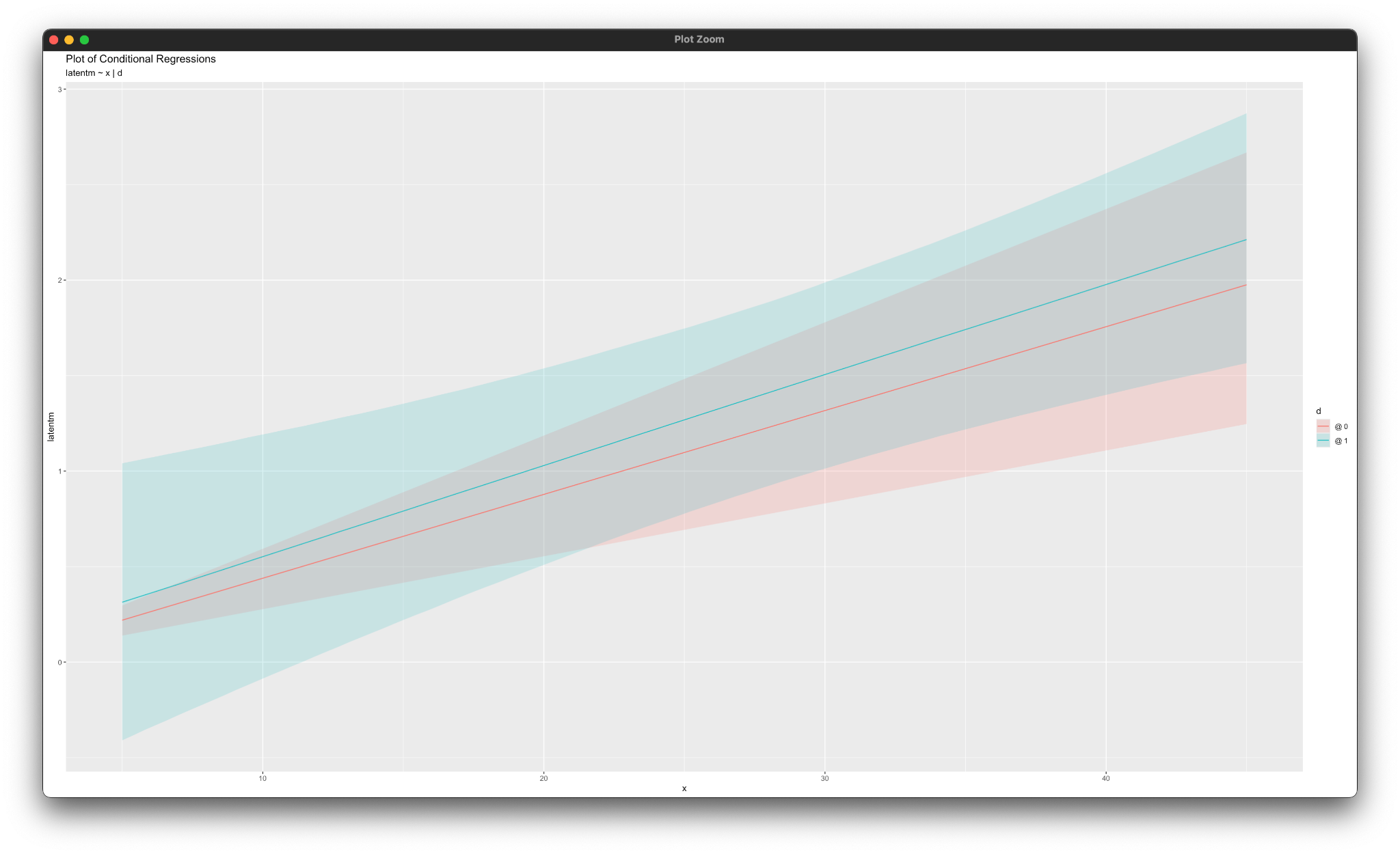
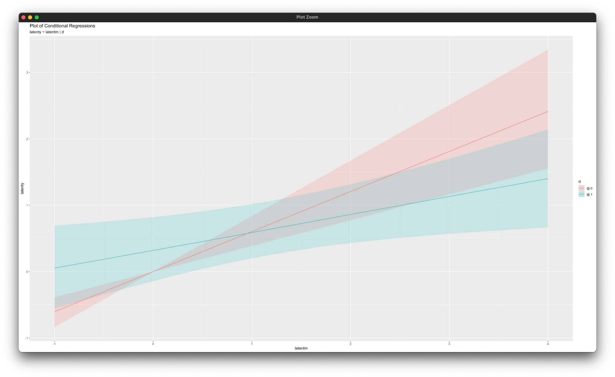
simple_plot(latentm ~ x | d, mymodel)
simple_plot(latenty ~ latentm | d, mymodel)

Working in rblimp is advantageous because graphing functions are available for visualizing results. For example, the simple_plot functions produce graphs of simple intercepts and slopes for x and latentm for each category of the moderator d, as shown below.

5.14 Moderated Nonlinear Factor Analysis (MNLFA)

This example illustrates a moderated nonlinear factor analysis (MNLFA). The method is conceptually similar to maximum likelihood MNLFA (Bauer, 2017) but does not require complicated nonlinear constraints. Instead, the model represents differential loadings (DIF) as an interaction between a latent variable and a manifest variable. In this example, the manifest variable is a grouping variable that predicts the factor’s mean and variance, and it also drives noninvariance in a loading and measurement intercept. The latent variable’s variance and the indicator variances can also be modeled as a function of the background variable, which does not need to be categorical. Enders, Vera, Keller, Lenartowicz, Loo (2024) describe Blimp’s MNLFA in detail and provide a real-data analysis example involving an integrative data analysis. The paper is available here, and the data analysis scripts for that more involved illustration are available at the paper’s OSF repository.

The measurement model equation for a given manifest indicator k is as follows.

\[y_k=\nu_{k}+\lambda_{k}\eta_y+\gamma_{1k}g+\gamma_{2k}(g)(\eta_y)+\varepsilon_k\]

The γ₁ slope is the effect of the covariate on the indicator’s mean, and the γ₂ interaction coefficient captures loading changes as a function of g. In this example, the indicators are continuous, but they could be any metric that Blimp supports. A path diagram of the model is shown below.

The straight lines from g to the indicators introduce group differences in measurement intercepts, and the dashed lines from g to the directed arrows reflect manifest-by-latent interaction terms (factor loading differences). Unlike a conventional multiple-group model, g could be a continuous dimension, although it is binary in this example. Finally, the model includes a log linear equation that relates the variance of the latent factor to the background variable.

\[\operatorname{ln}(\sigma_{\zeta}^2)=\omega_{0}+\omega_1g\]

For identification, the intercept 𝜔₀ is fixed at zero on the logarithmic metric, which sets the factor variance of the g = 0 group to 1. The 𝜔₁ coefficient captures the degree to which the factor variance differs on the log metric in group g = 1.

The syntax highlights are as follows.

ORDINAL command identifies a binary predictor
FIXED command identifies complete predictors (optional—speeds computation)
LATENT command defines a latent variable
Individual regression equations specified for each indicator (instead of the -> convention for latent factors)
MODEL command uses labels ending in a colon to group models and order their summary tables on the output
MODEL command labels intercept group differences and loading group differences
MODEL command features product terms
MODEL command uses an @ and a label to assign a positive-valued prior distribution to the first factor loading
MODEL command features a regression equation with the natural logarithm of the factor variance as the outcome
PARAMETER command defines a positive-valued uniform prior distribution
WALDTESTcommands specify Bayesian Wald tests that evaluate the null hypothesis that intercept and loading differences equal 0
SIMPLE command produces conditional effects (group-specific intercepts and loadings) at each level of the binary moderator
Longer burn-in period for estimating latent variables

DATA: data4.dat;
VARIABLES: id v1:v8 g y1:y6 v9:v21;
ORDINAL: g;
MISSING: 999;
FIXED: g;
LATENT: latenty;
MODEL:
  structural.model:
  latenty ~ 1@0 g;
  var(latenty) ~ 1@0 g;
  measurement.model:
  y1 ~ 1 latenty@load_prior;
  y2 ~ g@difficept1 latenty g*latenty@diffload1;
  y3 ~ g@difficept2 latenty g*latenty@diffload2;
  y4 ~ g@difficept3 latenty g*latenty@diffload3;
  y5 ~ g@difficept4 latenty g*latenty@diffload4;
  y6 ~ g@difficept5 latenty g*latenty@diffload5;
SIMPLE: latenty | g;
WALDTEST: diffload1:diffload5 = 0;
WALDTEST: difficept1:difficept5 = 0;
PARAMETERS:
  load_prior ~ truncate(0, Inf);
SEED: 90291;
BURN: 20000;
ITER: 20000;

The corresponding rblimp script is as follows. The simple_plot functions graph the simple intercepts and slopes from the measurement model.

library(rblimp)

mymodel <- rblimp(
  data = data,
  ordinal = 'g',
  fixed = 'g',
  latent = 'latenty',
  model = '
    structural.model:
    latenty ~ 1@0 g;
    var(latenty) ~ 1@0 g;
    measurement.model:
    y1 ~ 1 latenty@load_prior;
    y2 ~ g@difficept1 latenty g*latenty@diffload1;
    y3 ~ g@difficept2 latenty g*latenty@diffload2;
    y4 ~ g@difficept3 latenty g*latenty@diffload3;
    y5 ~ g@difficept4 latenty g*latenty@diffload4;
    y6 ~ g@difficept5 latenty g*latenty@diffload5',
  simple = 'latenty | g',
  waldtest = list('diffload1:diffload5 = 0','difficept1:difficept5 = 0'),
  parameters = 'load_prior ~ truncate(0, Inf)',
  seed = 90291,
  burn = 20000,
  iter = 20000
)

output(mymodel)
posterior_plot(mymodel)

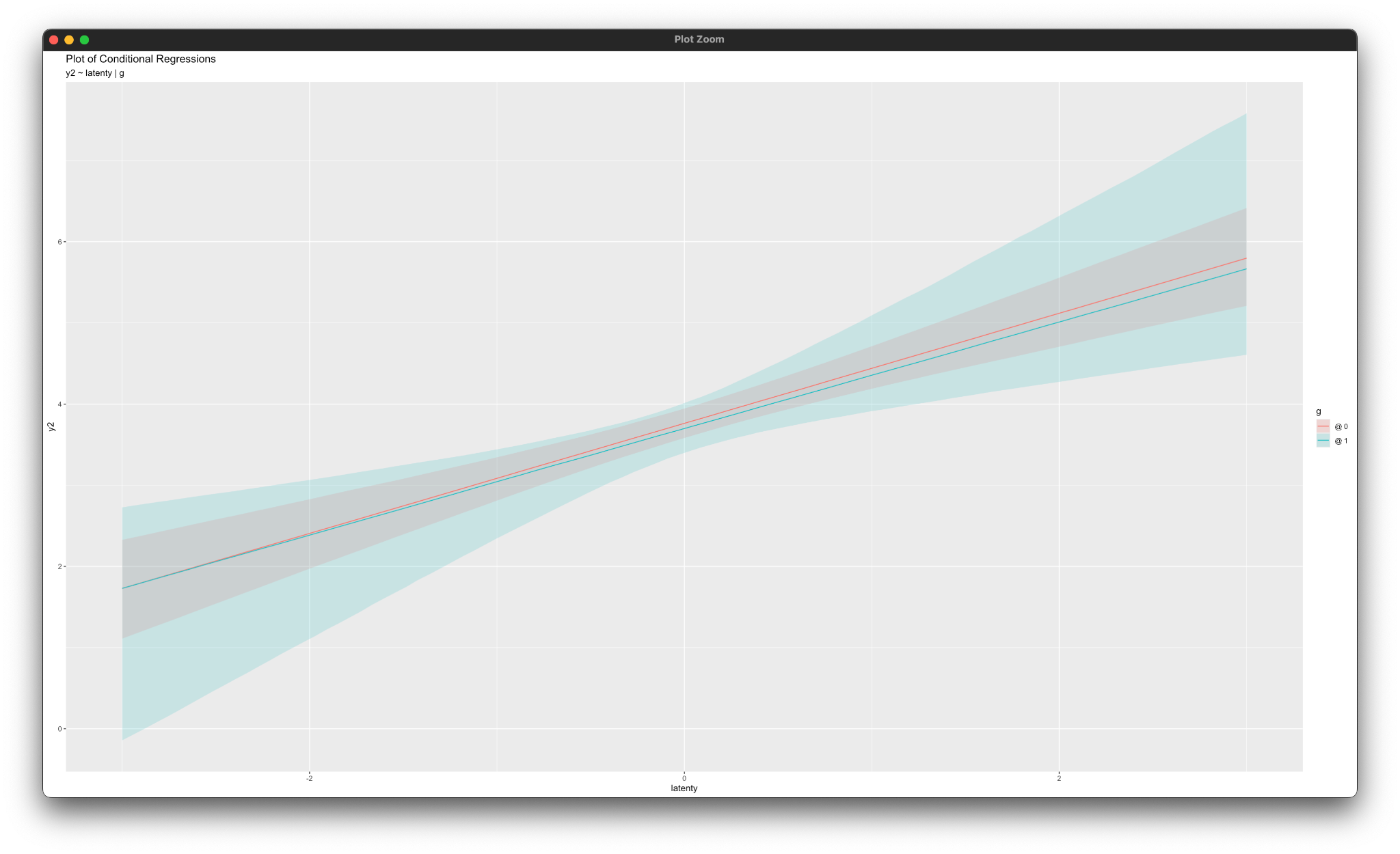
simple_plot(y2 ~ latenty | g, mymodel)
simple_plot(y3 ~ latenty | g, mymodel)
simple_plot(y4 ~ latenty | g, mymodel)
simple_plot(y5 ~ latenty | g, mymodel)
simple_plot(y6 ~ latenty | g, mymodel)

Working in rblimp is advantageous because graphing functions are available for visualizing results. For example, the simple_plot functions produce graphs of simple intercepts and factor loadings for latenty for each category of the moderator g, as shown below.

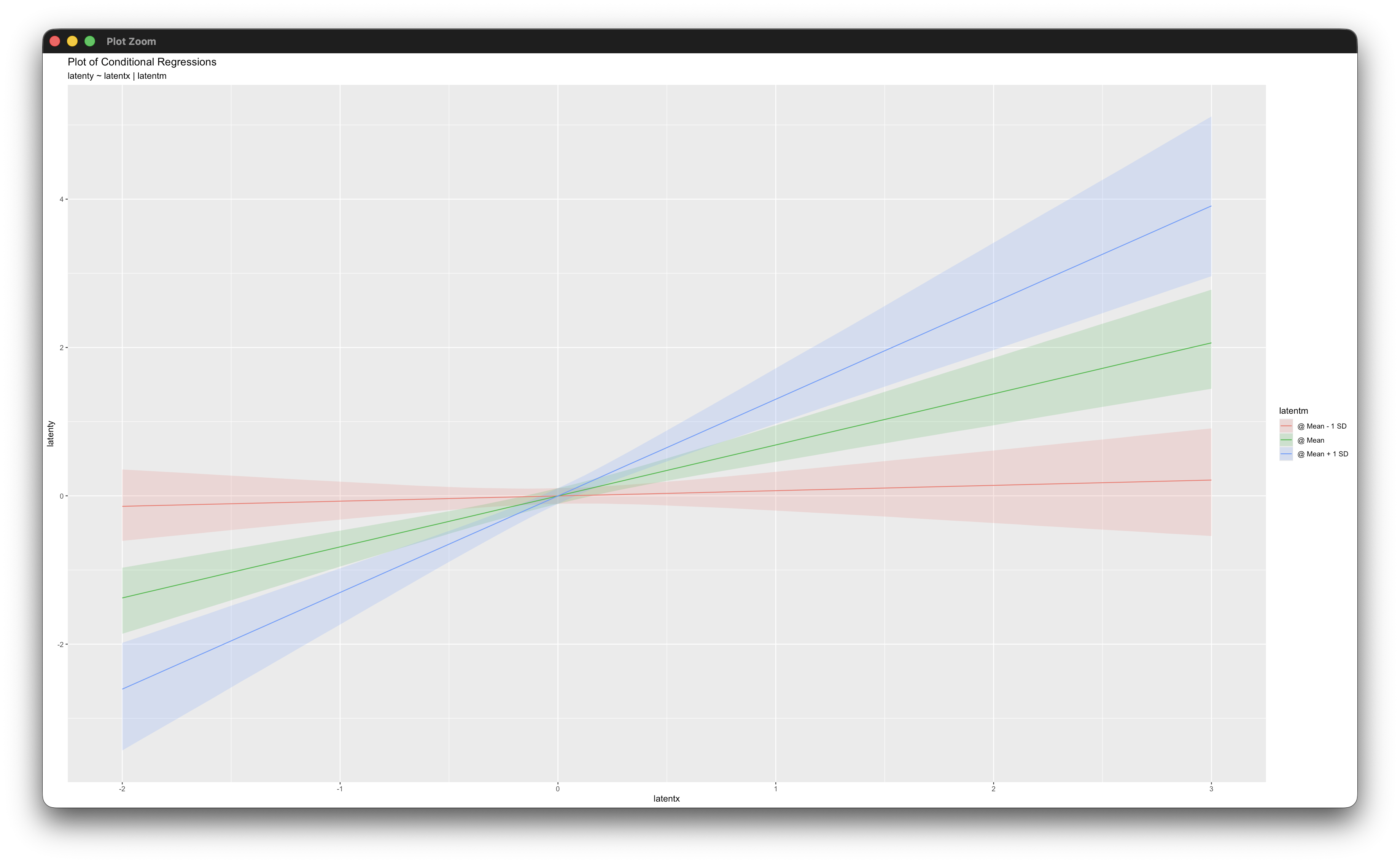
5.15 Latent-by-Latent Variable Interaction

Blimp can fit a broad range of latent variable interactions involving combinations of latent and manifest variables. The details on its interaction modeling are described in Keller (2025), which is available here. This example illustrates a latent variable regression model with two latent predictors and their interaction influencing a latent outcome variable. The structural regression equation is as follows.

\[\eta_y=\beta_0+\beta_1\eta_x+\beta_2\eta_m+\beta_3(\eta_x)(\eta_m)+\varepsilon\]

A path diagram of the full model is shown below.

The dashed line pointing from the latent variable to the directed arrow conveys that one latent predictor is moderating the influence of the other.

The syntax highlights are as follows.

ORDINAL command identifies ordinal variables
Automatic threshold specification for binary and ordinal variables
LATENT command defines three latent variables
MODEL command uses labels ending in a colon to group models and order their summary tables on the output
MODEL command features a two-way latent product term
MODEL command labels the structural regression slopes
MODEL command fixes variances and residual variances to one for identification
PARAMETERS command specifies a truncated prior over positive values, and the prior is attached to each factor’s first loading in the MODEL command
SIMPLE command produces conditional effects (simple slopes) at each three levels of the latent moderator

DATA: data13.dat;
VARIABLES: x1:x3 m1:m3 y1:y3;
MISSING: 999;
LATENT: latentx latentm latenty;
MODEL:
  structural.model:
  latenty ~ latentx latentm latentx*latentm;
  latenty ~~ latenty@1;
  predictor.model:
  latentx ~~ latentx@1;
  latentm ~~ latentm@1;
  latentx ~~ latentm;
  measurement.models:
  latentx -> x1@xload_prior x2:x3;
  latentm -> m1@mload_prior m2:m3;
  latenty -> y1@yload_prior y2:y3;
SIMPLE: latentx | latentm;
PARAMETERS:
  xload_prior ~ truncate(0, Inf);
  mload_prior ~ truncate(0, Inf);
  yload_prior ~ truncate(0, Inf);
SEED: 90291;
BURN: 10000;
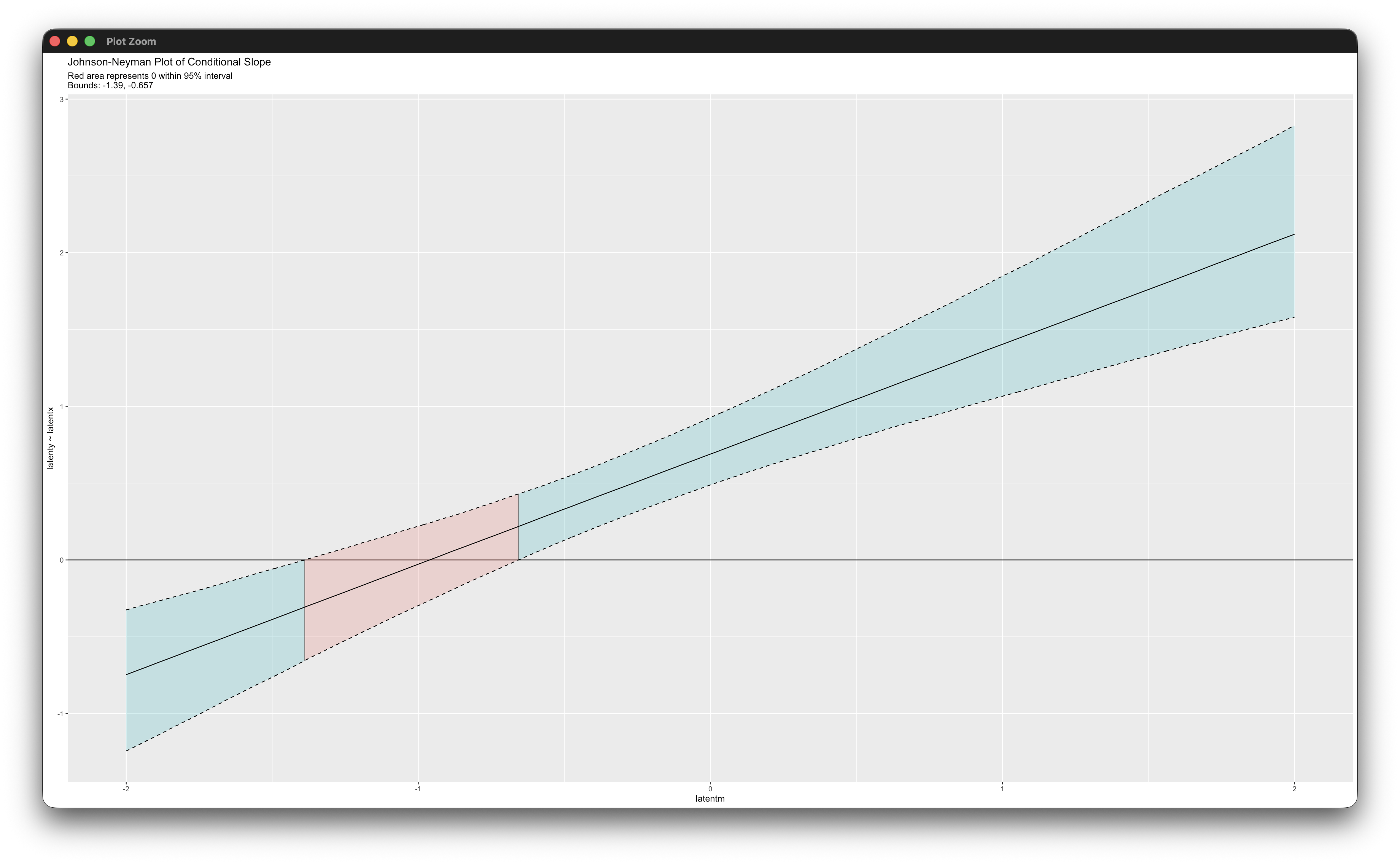
ITER: 10000;

The corresponding rblimp script is as follows. The simple_plot and jn_plot functions produce graphs of the simple intercepts and slopes and Johnson–Neyman regions of significance.

library(rblimp)

mymodel <- rblimp(
  data = data,
  latent = 'latentx latentm latenty',
  model = '
    structural.model:
    latenty ~ latentx latentm latentx*latentm;
    latenty ~~ latenty@1;
    predictor.model:
    latentx ~~ latentx@1;
    latentm ~~ latentm@1;
    latentx ~~ latentm;
    measurement.models:
    latentx -> x1@xload_prior x2:x3;
    latentm -> m1@mload_prior m2:m3;
    latenty -> y1@yload_prior y2:y3',
  simple = 'latentx | latentm',
  parameters = '
    xload_prior ~ truncate(0, Inf);
    mload_prior ~ truncate(0, Inf);
    yload_prior ~ truncate(0, Inf);',
  seed = 90291,
  burn = 10000,
  iter = 10000
)

output(mymodel)
posterior_plot(mymodel)

simple_plot(latenty ~ latentx | latentm, mymodel)
jn_plot(latenty ~ latentx | latentm, mymodel)

Working in rblimp is advantageous because graphing functions are available for visualizing results. The simple_plot function produces graphs of simple intercepts and slopes at three levels of the latent moderator, and the jn_plot displays Johnson–Neyman regions of significance.

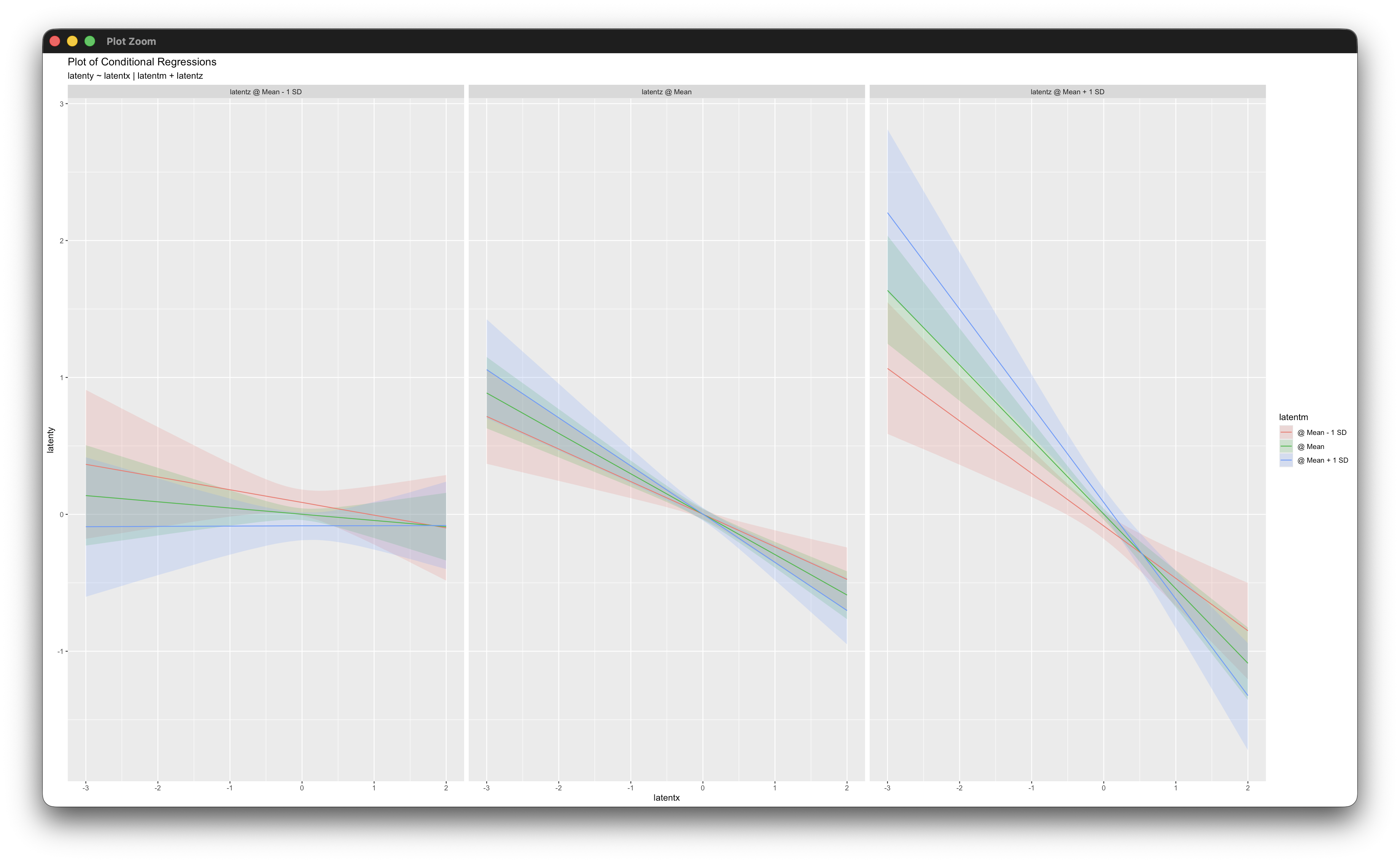
5.16 Three-Way Latent Variable Interaction

This example illustrates three-way interaction among latent variables. The procedure for the example is described in Keller (2025), which is available here. The structural model below corresponds to Equation 28 from the paper. We use established generic notation in lieu of the original variable names.

\[\eta_y=\beta_0+\beta_1\eta_x+\beta_2\eta_z+\beta_3\eta_m+\beta_4(\eta_x)(\eta_z)+\beta_5(\eta_x)(\eta_m)+\beta_6(\eta_z)(\eta_m)+\beta_7(\eta_x)(\eta_z)(\eta_m)+\varepsilon\]

The latent variables have 10 indicators each, and the indicators use 5-point rating scales. Following Example 5.9, the measurement models feature latent response variables regressed on the latent factors (probit regression).

The syntax highlights are as follows.

ORDINAL command identifies ordinal variables
Automatic threshold specification for binary and ordinal variables
LATENT command defines four latent variables
MODEL command uses labels ending in a colon to group models and order their summary tables on the output
MODEL command features two-way product terms and a three-way product
MODEL command labels the structural regression slopes
MODEL command fixes variances and residual variances to one for identification
PARAMETERS command specifies a truncated prior over positive values, and the prior is attached to each factor’s first loading in the MODEL command
SIMPLE command produces conditional effects (simple slopes) at multiple combinations of latent variables
Longer burn-in period and post-burn in iterations with ordinal variables

DATA: keller2024.dat;
VARIABLES: x1:x10 m1:m10 z1:z10 y1:y23 d1 d2;
ORDINAL: x1:x10 z1:z10 m1:m10 y1:y10;
LATENT: latentx latentm latentz latenty;
MODEL:
  structural.model:
  latenty ~ latentx@b1 latentz@b2 latentm@b3
    latentx*latentz@b4 latentx*latentm@b5 latentz*latentm@b6
    latentx*latentz*latentm@b7;
  latenty@1;
  predictor.model:
  latentx latentz latentm ~~ latentx latentz latentm;
  latentx@1;
  latentz@1;
  latentm@1;
  measurement.models:
  latentx -> x1@xload_prior x2:x10;
  latentz -> z1@zload_prior z2:z10;
  latentm -> m1@mload_prior m2:m10;
  latenty -> y1@yload_prior y2:y10;
SIMPLE: latentx | latentm and latentz;
PARAMETERS:
  xload_prior ~ truncate(0, Inf);
  zload_prior ~ truncate(0, Inf);
  mload_prior ~ truncate(0, Inf);
  yload_prior ~ truncate(0, Inf);
SEED: 90291;
BURN: 50000;
ITER: 50000;

The corresponding rblimp script is as follows.

library(rblimp)

mymodel <- rblimp(
  data = data,
  ordinal = 'x1:x10 z1:z10 m1:m10 y1:y10',
  latent = 'latentx latentm latentz latenty',
  model = '
    structural.model:
    latenty ~ latentx@b1 latentz@b2 latentm@b3
      latentx*latentz@b4 latentx*latentm@b5 latentz*latentm@b6
      latentx*latentz*latentm@b7;
    latenty@1;
    predictor.model:
    latentx latentz latentm ~~ latentx latentz latentm;
    latentx@1;
    latentz@1;
    latentm@1;
    measurement.models:
    latentx -> x1@xload_prior x2:x10;
    latentz -> z1@zload_prior z2:z10;
    latentm -> m1@mload_prior m2:m10;
    latenty -> y1@yload_prior y2:y10',
  simple = 'latentx | latentm and latentz',
  parameters = '
    xload_prior ~ truncate(0, Inf);
    zload_prior ~ truncate(0, Inf);
    mload_prior ~ truncate(0, Inf);
    yload_prior ~ truncate(0, Inf);',
  seed = 90291,
  burn = 50000,
  iter = 50000
)

output(mymodel)
posterior_plot(mymodel)
simple_plot(latenty ~ latentx | latentm and latentz, mymodel)

Working in rblimp is advantageous because graphing functions are available for visualizing results. The simple_plot function produces graphs of simple intercepts and slopes at combinations of three levels of each latent moderator.

5.17 Latent Growth Curve Model

This example illustrates a two-factor latent growth curve model with unequally spaced repeated measurements and a binary predictor of the random intercepts and slopes. A path diagram of the model is shown below.

The syntax highlights are as follows.

ORDINALcommand identifies a binary predictor
FIXEDcommand identifies complete predictors
LATENT command defines two latent variables
MODEL command uses labels ending in a colon to group models and order their summary tables on the output
Individual regression equations specified for each indicator (instead of the -> convention for latent factors)
MODEL command uses the -> convention to add random intercepts and slopes as a predictor to each measurement model and fix the loadings and measurement intercepts
MODEL command estimates the latent variable means, fixes the intercept factor loadings to one, fixes the growth factor loadings to the time scores (0, 1, 3, and 6), and fixes the measurement intercepts to zero
MODEL command uses a label to impose equality constraint on residual variance

DATA: data3.dat;
VARIABLES: id y0 y1 y3 y6 d v1:v5;
ORDINAL: d;
MISSING: 999;
FIXED: d;
LATENT: eta_icept eta_slope;
MODEL:
  structural.model:
  eta_icept ~ 1 d;
  eta_slope ~ 1 d;
  eta_icept ~~ eta_slope;
  measurement.model:
  eta_icept -> y0@1 y1@1 y3@1 y6@1;
  eta_slope -> y0@0 y1@1 y3@3 y6@6;
  1 -> y0@0 y1@0 y3@0 y6@0;
  # common residual variance
  y0@resvar;
  y1@resvar;
  y3@resvar;
  y6@resvar;
SEED: 90291;
BURN: 10000;
ITER: 10000;

The corresponding rblimp script is as follows.

library(rblimp)

mymodel <- rblimp(
  data = data,
  ordinal = 'd',
  fixed = 'd',
  latent = 'eta_icept eta_slope',
  model = '
    structural.model:
    eta_icept ~ 1 d;
    eta_slope ~ 1 d;
    eta_icept ~~ eta_slope;
    measurement.model:
    eta_icept -> y0@1 y1@1 y3@1 y6@1;
    eta_slope -> y0@0 y1@1 y3@3 y6@6;
    1 -> y0@0 y1@0 y3@0 y6@0;
    # common residual variance
    y0@resvar;
    y1@resvar;
    y3@resvar;
    y6@resvar;',
  seed = 90291,
  burn = 10000,
  iter = 10000
)

output(mymodel)
posterior_plot(mymodel)

5.18 Residual SEM: AR1 Growth Model

This example illustrates a residual SEM that specifies an AR1 structure on the residuals in a latent growth curve model. The model features the residuals at each time point predicting the outcome at the next measurement occasion. The path diagram below shows a growth model with six waves of data. The residual variables that comprise the AR1 structure are computed by subtracting the predicted value from the observed value.

\[ry_{1} = y_{1} - (\eta_{icept} + 0\eta_{slope})\]

\[ry_{2} = y_{2} - (\eta_{icept} + 1\eta_{slope})\]

\[ry_{3} = y_{3} - (\eta_{icept} + 2\eta_{slope})\]

\[ry_{4} = y_{4} - (\eta_{icept} + 3\eta_{slope})\]

\[ry_{5} = y_{5} - (\eta_{icept} + 4\eta_{slope})\]

Note that the residual variables (the rys) are not themselves random variables. Rather, they are simply functions defined by centering each repeated measures variable at its predicted value using the estimated random intercepts and slopes.

The syntax highlights are as follows.

LATENT command defines two latent variables that represent person-specific random intercepts and slopes
MODEL command uses definition variables that specify the residual computations, and it uses those definitions as predictors in the measurement models
MODEL command uses labels ending in a colon to group models and order their summary tables on the output
MODEL command uses the -> convention to add random intercepts and slopes as a predictor to each measurement model and fix the loadings and measurement intercepts
MODEL command estimates the latent variable means, fixes the intercept factor loadings to one, fixes the growth factor loadings to integer values between zero and six
WALDTESTcommand invokes a Bayesian Wald test that evaluates the null hypothesis that the autocorrelations are equal

DATA: data27.dat;
VARIABLES: y1:y6 z;
MISSING: 999;
LATENT: eta_icept eta_slope;
MODEL:
  # definition variables for residuals
  ry1 = y1 - (eta_icept + (0*eta_slope));
  ry2 = y2 - (eta_icept + (1*eta_slope));
  ry3 = y3 - (eta_icept + (2*eta_slope));
  ry4 = y4 - (eta_icept + (3*eta_slope));
  ry5 = y5 - (eta_icept + (4*eta_slope));
  structural.model:
  eta_icept ~~ eta_slope;
  1 -> eta_icept eta_slope;
  measurement.model:
  eta_icept -> y1@1 y2@1 y3@1 y4@1 y5@1 y6@1;
  eta_slope -> y1@0 y2@1 y3@2 y4@3 y5@4 y6@5;
  1 -> y1@0 y2@0 y3@0 y4@0 y5@0 y6@0;
  # AR1 paths
  y2 ~ ry1@ac1;
  y3 ~ ry2@ac2;
  y4 ~ ry3@ac3;
  y5 ~ ry4@ac4;
  y6 ~ ry5@ac5;
WALDTEST: ac1 = ac2:ac5;
SEED: 90291;
BURN: 30000;
ITER: 30000;

The corresponding rblimp script is as follows.

library(rblimp)

mymodel <- rblimp(
  data = data,
  latent = 'eta_icept eta_slope',
  model = '
    # definition variables for residuals
    ry1 = y1 - (eta_icept + (0*eta_slope));
    ry2 = y2 - (eta_icept + (1*eta_slope));
    ry3 = y3 - (eta_icept + (2*eta_slope));
    ry4 = y4 - (eta_icept + (3*eta_slope));
    ry5 = y5 - (eta_icept + (4*eta_slope));
    structural.model:
    eta_icept ~~ eta_slope;
    1 -> eta_icept eta_slope;
    measurement.model:
    eta_icept -> y1@1 y2@1 y3@1 y4@1 y5@1 y6@1;
    eta_slope -> y1@0 y2@1 y3@2 y4@3 y5@4 y6@5;
    1 -> y1@0 y2@0 y3@0 y4@0 y5@0 y6@0;
    # AR1 paths
    y2 ~ ry1@ac1;
    y3 ~ ry2@ac2;
    y4 ~ ry3@ac3;
    y5 ~ ry4@ac4;
    y6 ~ ry5@ac5;',
  waldtest = 'ac1 = ac2:ac5',
  seed = 90291,
  burn = 30000,
  iter = 30000
)

output(mymodel)
posterior_plot(mymodel)

MODEL:
  # define residuals
  { i in 1:5 } : ry[i] = y[i] - (eta_icept + ([i-1] * eta_slope));
  structural.model:
  eta_icept ~~ eta_slope;
  1 -> eta_icept eta_slope;
  measurement.model:
  y1 ~ 1@eta_icept eta_slope@0;
  { i in 2:6 } : y[i] ~ 1@eta_icept eta_slope@[i-1] ry[i-1]@ac[i-1];

The first loop defines occasion-specific residual variables ry[i]. The index i ranges from 1 to 5, and for each value the loop subtracts the predicted value—defined by the random intercept, a loop-defined time score [i-1], and a random slope—from the observed outcome y[i]. In the measurement model section, the index i ranges from 2 to 6 and is used to select the outcome variable, define a slope factor loading, select a residual variable, and assign a label.

The MCMC Wald test was not significant, indicating that a simpler model where all autocorrelation paths are equal is preferable. The code block below illustrates equality constraints on the residual associations.

DATA: data27.dat;
VARIABLES: y1:y6 z;
MISSING: 999;
LATENT: eta_icept eta_slope;
MODEL:
  # definition variables for residuals
  ry1 = y1 - (eta_icept + (0*eta_slope));
  ry2 = y2 - (eta_icept + (1*eta_slope));
  ry3 = y3 - (eta_icept + (2*eta_slope));
  ry4 = y4 - (eta_icept + (3*eta_slope));
  ry5 = y5 - (eta_icept + (4*eta_slope));
  structural.model:
  eta_icept ~~ eta_slope;
  1 -> eta_icept eta_slope;
  measurement.model:
  eta_icept -> y1@1 y2@1 y3@1 y4@1 y5@1 y6@1;
  eta_slope -> y1@0 y2@1 y3@2 y4@3 y5@4 y6@5;
  1 -> y1@0 y2@0 y3@0 y4@0 y5@0 y6@0;
  # AR1 paths
  y2 ~ ry1@ac;
  y3 ~ ry2@ac;
  y4 ~ ry3@ac;
  y5 ~ ry4@ac;
  y6 ~ ry5@ac;
SEED: 90291;
BURN: 20000;
ITER: 20000;

The corresponding rblimp script is as follows.

library(rblimp)

mymodel <- rblimp(
  data = data,
  latent = 'eta_icept eta_slope',
  model = '
    # definition variables for residuals
    ry1 = y1 - (eta_icept + (0*eta_slope));
    ry2 = y2 - (eta_icept + (1*eta_slope));
    ry3 = y3 - (eta_icept + (2*eta_slope));
    ry4 = y4 - (eta_icept + (3*eta_slope));
    ry5 = y5 - (eta_icept + (4*eta_slope));
    structural.model:
    eta_icept ~~ eta_slope;
    1 -> eta_icept eta_slope;
    measurement.model:
    eta_icept -> y1@1 y2@1 y3@1 y4@1 y5@1 y6@1;
    eta_slope -> y1@0 y2@1 y3@2 y4@3 y5@4 y6@5;
    1 -> y1@0 y2@0 y3@0 y4@0 y5@0 y6@0;
    # AR1 paths
    y2 ~ ry1@ac;
    y3 ~ ry2@ac;
    y4 ~ ry3@ac;
    y5 ~ ry4@ac;
    y6 ~ ry5@ac;',
  seed = 90291,
  burn = 20000,
  iter = 20000
)

output(mymodel)
posterior_plot(mymodel)

As before, Blimp offers a looping structure within the MODEL command that allows repetitive features of a model more concisely in fewer lines of code. The MODEL and PARAMETERS section of the script can be specified more concisely as follows.

MODEL:
  # define residuals
  { i in 1:5 } : ry[i] = y[i] - (eta_icept + ([i-1] * eta_slope));
  structural.model:
  eta_icept ~~ eta_slope;
  1 -> eta_icept eta_slope;
  measurement.model:
  y1 ~ 1@eta_icept eta_slope@0;
  { i in 2:6 } : y[i] ~ 1@eta_icept eta_slope@[i-1] ry[i-1]@ac;

5.19 Random Intercept Cross-Lagged Panel Model (RI-CLPM)

This example illustrates a random intercept cross-lagged panel model. The analysis and the data are from Mulder and Hamaker (2021). The simulated data were obtained from the paper’s website. The basic RI-CLPM is described in Hamaker, Kuiper, and Grasman (2015). The model features a random intercept latent variable that removes stable individual differences from the lagged processes, which represent pure within-person effects. The path diagram below shows a three-wave version of the model.

The rx and ry variables in oval denote within-person residuals. The cross-lagged paths are defined as within-person slopes because the manifest variables are centered at the random intercepts, thus removing stable between-person variation. The residuals are computed as follows.

\[rx_{1} = x_{1} - (\mu_{x1} + \eta_x)\]

\[rx_{2} = x_{2} - (\mu_{x2} + \eta_x)\]

\[ry_{1} = y_{1} - (\mu_{y1} + \eta_y)\]

\[ry_{2} = y_{2} - (\mu_{y2}+\eta_y)\]

In Blimp, the residuals (the rxs and rys) are not themselves random variables. Rather, they are simply functions defined by centering each repeated measures variable at the estimated random intercept. Finally, the residual variances and covariances are within-person effects by virtue of the random intercept latent variable removing stable between-person variation.

The syntax highlights are as follows.

LATENT command defines two latent variables that represent person-specific random intercepts for the two variables
MODEL command uses labels ending in a colon to group models and order their summary tables on the output
MODEL command leverages Blimp’s default, which is to set latent variable means equal to zero
MODEL command sets the random intercept latent variable’s factor loadings to one
MODEL command creates pure within-person predictors by centering each person’s scores at their random intercept estimates
MODEL command uses definition variables that specify the residual computations, and it uses those definitions as predictors in the measurement models

DATA: RICLPM.dat;
VARIABLES: x1:x5 y1:y5 z2 z1;
LATENT: etax etay;
MODEL:
  # definition variables for residuals
  rx1 = x1 - (mux1 + etax);
  rx2 = x2 - (mux2 + etax);
  rx3 = x3 - (mux3 + etax);
  rx4 = x4 - (mux4 + etax);
  ry1 = y1 - (muy1 + etay);
  ry2 = y2 - (muy2 + etay);
  ry3 = y3 - (muy3 + etay);
  ry4 = y4 - (muy4 + etay);
  random.intercepts:
  etax ~~ etay;
  x.models:
  x1 ~ 1@mux1 etax@1;
  x2 ~ 1@mux2 etax@1 rx1 ry1;
  x3 ~ 1@mux3 etax@1 rx2 ry2;
  x4 ~ 1@mux4 etax@1 rx3 ry3;
  x5 ~ 1@mux5 etax@1 rx4 ry4;
  y.models:
  y1 ~ 1@muy1 etay@1;
  y2 ~ 1@muy2 etay@1 ry1 rx1;
  y3 ~ 1@muy3 etay@1 ry2 rx2;
  y4 ~ 1@muy4 etay@1 ry3 rx3;
  y5 ~ 1@muy5 etay@1 ry4 rx4;
  covariances:
  x1 ~~ y1;
  x2 ~~ y2;
  x3 ~~ y3;
  x4 ~~ y4;
  x5 ~~ y5;
SEED: 90291;
BURN: 10000;
ITER: 10000;

The corresponding rblimp script is as follows.

library(rblimp)

mymodel <- rblimp(
  data = data,
  latent = 'etax etay',
  model = '
    # definition variables for residuals
    rx1 = x1 - (mux1 + etax);
    rx2 = x2 - (mux2 + etax);
    rx3 = x3 - (mux3 + etax);
    rx4 = x4 - (mux4 + etax);
    ry1 = y1 - (muy1 + etay);
    ry2 = y2 - (muy2 + etay);
    ry3 = y3 - (muy3 + etay);
    ry4 = y4 - (muy4 + etay);
    random.intercepts:
    etax ~~ etay;
    x.models:
    x1 ~ 1@mux1 etax@1;
    x2 ~ 1@mux2 etax@1 rx1 ry1;
    x3 ~ 1@mux3 etax@1 rx2 ry2;
    x4 ~ 1@mux4 etax@1 rx3 ry3;
    x5 ~ 1@mux5 etax@1 rx4 ry4;
    y.models:
    y1 ~ 1@muy1 etay@1;
    y2 ~ 1@muy2 etay@1 ry1 rx1;
    y3 ~ 1@muy3 etay@1 ry2 rx2;
    y4 ~ 1@muy4 etay@1 ry3 rx3;
    y5 ~ 1@muy5 etay@1 ry4 rx4;
    covariances:
    x1 ~~ y1;
    x2 ~~ y2;
    x3 ~~ y3;
    x4 ~~ y4;
    x5 ~~ y5;',
  seed = 90291,
  burn = 10000,
  iter = 10000
)

output(mymodel)
posterior_plot(mymodel)

MODEL:
  # define residuals
  { v in x y, i in 1:4 } : r[v][i] = [v][i] - (mu[v][i] + eta[v]);
  random.intercept:
  etax ~~ etay;
  x.models:
  x1 ~ 1@mux1 etax@1;
  { i in 2:5 } : x[i] ~ 1@mux[i] etax@1 rx[i-1] ry[i-1];
  y.models:
  y1 ~ 1@muy1 etay@1;
  { i in 2:5 } : y[i] ~ 1@muy[i] etay@1 ry[i-1] rx[i-1];
  covariances:
  { i in 1:5 } : x[i] ~~ y[i];

The first loop uses two iteration indices—v over the variable names x and y, and i over occasions 1 through 4—to define residuals. For each combination of v and i, the loop subtracts the predicted value, defined by the variable- and time-specific mean mu[v][i] and the corresponding random intercept eta[v], from the observed value [v][i], generating residuals r[v][i]. In the x.models and y.models blocks, the i index ranges from 2 to 5 and is used to generate lagged regression equations across time. The index selects the current outcome (x[i] or y[i]), the corresponding mean parameter, and the appropriate lagged residuals from the previous occasion ([i-1]). The final loop, indexed by i from 1 to 5, specifies contemporaneous covariances between x[i] and y[i] at each time point, generating one covariance per occasion.

Mulder and Hamaker (2021) describe four extensions of the RI-CLPM. The first introduces a time-invariant covariate predicting the repeated measures variables. The residual variables that appear as predictors in the models are now computed by subtracting out the random intercept plus the effect of z1 as follows.

\[rx_{1} = x_{1} - [\mu_{x1}+\eta_x+\alpha_1(z_1)]\]

\[rx_{2} = x_{2} - [\mu_{x2}+\eta_x+\alpha_2(z_1)]\]

\[ry_{1} = y_{1} - [\mu_{y1}+\eta_y+\beta_1(z_1)]\]

\[ry_{2} = y_{2} - [\mu_{y2}+\eta_y+\beta_2(z_1)]\]

The Blimp script for this five-wave analysis is shown below. The binary covariate z1 is identified on the ORDINAL line to invoke probit regression in the event of missing data.

DATA: RICLPM.dat;
VARIABLES: x1:x5 y1:y5 z2 z1;
ORDINAL: z1;
LATENT: etax etay;
MODEL:
  # definition variables for residuals
  rx1 = x1 - (mux1 + etax + z1*a1);
  rx2 = x2 - (mux2 + etax + z1*a2);
  rx3 = x3 - (mux3 + etax + z1*a3);
  rx4 = x4 - (mux4 + etax + z1*a4);
  ry1 = y1 - (muy1 + etay + z1*b1);
  ry2 = y2 - (muy2 + etay + z1*b2);
  ry3 = y3 - (muy3 + etay + z1*b3);
  ry4 = y4 - (muy4 + etay + z1*b4);
  random.intercepts:
  etax ~~ etay;
  x.models:
  x1 ~ 1@mux1 etax@1 z1@a1;
  x2 ~ 1@mux2 etax@1 rx1 ry1 z1@a2;
  x3 ~ 1@mux3 etax@1 rx2 ry2 z1@a3;
  x4 ~ 1@mux4 etax@1 rx3 ry3 z1@a4;
  x5 ~ 1@mux5 etax@1 rx4 ry4 z1@a5;
  y.models:
  y1 ~ 1@muy1 etay@1 z1@b1;
  y2 ~ 1@muy2 etay@1 ry1 rx1 z1@b2;
  y3 ~ 1@muy3 etay@1 ry2 rx2 z1@b3;
  y4 ~ 1@muy4 etay@1 ry3 rx3 z1@b4;
  y5 ~ 1@muy5 etay@1 ry4 rx4 z1@b5;
  covariances:
  x1 ~~ y1;
  x2 ~~ y2;
  x3 ~~ y3;
  x4 ~~ y4;
  x5 ~~ y5;
SEED: 90291;
BURN: 10000;
ITER: 10000;

The corresponding rblimp script is as follows.

library(rblimp)

mymodel <- rblimp(
  data = data,
  ordinal = 'z1',
  latent = 'etax etay',
  model = '
    # definition variables for residuals
    rx1 = x1 - (mux1 + etax + z1*a1);
    rx2 = x2 - (mux2 + etax + z1*a2);
    rx3 = x3 - (mux3 + etax + z1*a3);
    rx4 = x4 - (mux4 + etax + z1*a4);
    ry1 = y1 - (muy1 + etay + z1*b1);
    ry2 = y2 - (muy2 + etay + z1*b2);
    ry3 = y3 - (muy3 + etay + z1*b3);
    ry4 = y4 - (muy4 + etay + z1*b4);
    random.intercepts:
    etax ~~ etay;
    x.models:
    x1 ~ 1@mux1 etax@1 z1@a1;
    x2 ~ 1@mux2 etax@1 rx1 ry1 z1@a2;
    x3 ~ 1@mux3 etax@1 rx2 ry2 z1@a3;
    x4 ~ 1@mux4 etax@1 rx3 ry3 z1@a4;
    x5 ~ 1@mux5 etax@1 rx4 ry4 z1@a5;
    y.models:
    y1 ~ 1@muy1 etay@1 z1@b1;
    y2 ~ 1@muy2 etay@1 ry1 rx1 z1@b2;
    y3 ~ 1@muy3 etay@1 ry2 rx2 z1@b3;
    y4 ~ 1@muy4 etay@1 ry3 rx3 z1@b4;
    y5 ~ 1@muy5 etay@1 ry4 rx4 z1@b5;
    covariances:
    x1 ~~ y1;
    x2 ~~ y2;
    x3 ~~ y3;
    x4 ~~ y4;
    x5 ~~ y5;',
  seed = 90291,
  burn = 10000,
  iter = 10000
)

output(mymodel)
posterior_plot(mymodel)

MODEL:
  # define residuals
  { v in x y, i in 1:4 } : r[v][i] = [v][i] - (mu[v][i] + eta[v] + z1*b[v][i]);
  random.intercept:
  etax ~~ etay;
  x.models:
  x1 ~ 1@mux1 etax@1 z1@bx1;
  { i in 2:5 } : x[i] ~ 1@mux[i] etax@1 rx[i-1] ry[i-1] z1@bx[i];
  y.models:
  y1 ~ 1@muy1 etay@1 z1@by1;
  { i in 2:5 } : y[i] ~ 1@muy[i] etay@1 ry[i-1] rx[i-1] z1@by[i];
  covariances:
  { i in 1:5 } : x[i] ~~ y[i];

The remaining examples in this section can be simplified using the same looping strategy.

The second extension introduces a covariate predicting the random intercept latent variables. Mulder and Hamaker (2021) note that this model is statistically equivalent to one that places equality constraints on the z1 slopes from the previous example. The Blimp script for this analysis is shown below. The binary covariate z1 is identified on the ORDINAL line to invoke probit regression in the event of missing data.

DATA: RICLPM.dat;
VARIABLES: x1:x5 y1:y5 z2 z1;
ORDINAL: z1;
LATENT: etax etay;
MODEL:
  # definition variables for residuals
  rx1 = x1 - (mux1 + etax);
  rx2 = x2 - (mux2 + etax);
  rx3 = x3 - (mux3 + etax);
  rx4 = x4 - (mux4 + etax);
  ry1 = y1 - (muy1 + etay);
  ry2 = y2 - (muy2 + etay);
  ry3 = y3 - (muy3 + etay);
  ry4 = y4 - (muy4 + etay);
  random.intercepts:
  etax ~ z1;
  etay ~ z1;
  etax ~~ etay;
  x.models:
  x1 ~ 1@mux1 etax@1;
  x2 ~ 1@mux2 etax@1 rx1 ry1;
  x3 ~ 1@mux3 etax@1 rx2 ry2;
  x4 ~ 1@mux4 etax@1 rx3 ry3;
  x5 ~ 1@mux5 etax@1 rx4 ry4;
  y.models:
  y1 ~ 1@muy1 etay@1;
  y2 ~ 1@muy2 etay@1 ry1 rx1;
  y3 ~ 1@muy3 etay@1 ry2 rx2;
  y4 ~ 1@muy4 etay@1 ry3 rx3;
  y5 ~ 1@muy5 etay@1 ry4 rx4;
  covariances:
  x1 ~~ y1;
  x2 ~~ y2;
  x3 ~~ y3;
  x4 ~~ y4;
  x5 ~~ y5;
SEED: 90291;
BURN: 10000;
ITER: 10000;

The corresponding rblimp script is as follows.

library(rblimp)

mymodel <- rblimp(
  data = data,
  latent = 'etax etay',
  ordinal = 'z1',
  model = '
    # definition variables for residuals
    rx1 = x1 - (mux1 + etax);
    rx2 = x2 - (mux2 + etax);
    rx3 = x3 - (mux3 + etax);
    rx4 = x4 - (mux4 + etax);
    ry1 = y1 - (muy1 + etay);
    ry2 = y2 - (muy2 + etay);
    ry3 = y3 - (muy3 + etay);
    ry4 = y4 - (muy4 + etay);
    random.intercepts:
    etax ~ z1;
    etay ~ z1;
    etax ~~ etay;
    x.models:
    x1 ~ 1@mux1 etax@1;
    x2 ~ 1@mux2 etax@1 rx1 ry1;
    x3 ~ 1@mux3 etax@1 rx2 ry2;
    x4 ~ 1@mux4 etax@1 rx3 ry3;
    x5 ~ 1@mux5 etax@1 rx4 ry4;
    y.models:
    y1 ~ 1@muy1 etay@1;
    y2 ~ 1@muy2 etay@1 ry1 rx1;
    y3 ~ 1@muy3 etay@1 ry2 rx2;
    y4 ~ 1@muy4 etay@1 ry3 rx3;
    y5 ~ 1@muy5 etay@1 ry4 rx4;
    covariances:
    x1 ~~ y1;
    x2 ~~ y2;
    x3 ~~ y3;
    x4 ~~ y4;
    x5 ~~ y5;',
  seed = 90291,
  burn = 10000,
  iter = 10000
)

output(mymodel)

The third and fourth extensions feature a distal outcome, z2. This outcome can be regressed on the random intercepts and/or the within-person predictors. The script below features the random intercepts predicting the distal outcome.

DATA: RICLPM.dat;
VARIABLES: x1:x5 y1:y5 z2 z1;
LATENT: etax etay;
MODEL:
  # definition variables for residuals
  rx1 = x1 - (mux1 + etax);
  rx2 = x2 - (mux2 + etax);
  rx3 = x3 - (mux3 + etax);
  rx4 = x4 - (mux4 + etax);
  ry1 = y1 - (muy1 + etay);
  ry2 = y2 - (muy2 + etay);
  ry3 = y3 - (muy3 + etay);
  ry4 = y4 - (muy4 + etay);
  random.intercepts:
  etax ~~ etay;
  x.models:
  x1 ~ 1@mux1 etax@1;
  x2 ~ 1@mux2 etax@1 rx1 ry1;
  x3 ~ 1@mux3 etax@1 rx2 ry2;
  x4 ~ 1@mux4 etax@1 rx3 ry3;
  x5 ~ 1@mux5 etax@1 rx4 ry4;
  y.models:
  y1 ~ 1@muy1 etay@1;
  y2 ~ 1@muy2 etay@1 ry1 rx1;
  y3 ~ 1@muy3 etay@1 ry2 rx2;
  y4 ~ 1@muy4 etay@1 ry3 rx3;
  y5 ~ 1@muy5 etay@1 ry4 rx4;
  covariances:
  x1 ~~ y1;
  x2 ~~ y2;
  x3 ~~ y3;
  x4 ~~ y4;
  x5 ~~ y5;
  distal.outcome:
  z2 ~ etax etay;
SEED: 90291;
BURN: 10000;
ITER: 10000;

The corresponding rblimp script is as follows.

library(rblimp)

mymodel <- rblimp(
  data = data,
  latent = 'etax etay',
  model = '
    # definition variables for residuals
    rx1 = x1 - (mux1 + etax);
    rx2 = x2 - (mux2 + etax);
    rx3 = x3 - (mux3 + etax);
    rx4 = x4 - (mux4 + etax);
    ry1 = y1 - (muy1 + etay);
    ry2 = y2 - (muy2 + etay);
    ry3 = y3 - (muy3 + etay);
    ry4 = y4 - (muy4 + etay);
    random.intercepts:
    etax ~~ etay;
    x.models:
    x1 ~ 1@mux1 etax@1;
    x2 ~ 1@mux2 etax@1 rx1 ry1;
    x3 ~ 1@mux3 etax@1 rx2 ry2;
    x4 ~ 1@mux4 etax@1 rx3 ry3;
    x5 ~ 1@mux5 etax@1 rx4 ry4;
    y.models:
    y1 ~ 1@muy1 etay@1;
    y2 ~ 1@muy2 etay@1 ry1 rx1;
    y3 ~ 1@muy3 etay@1 ry2 rx2;
    y4 ~ 1@muy4 etay@1 ry3 rx3;
    y5 ~ 1@muy5 etay@1 ry4 rx4;
    covariances:
    x1 ~~ y1;
    x2 ~~ y2;
    x3 ~~ y3;
    x4 ~~ y4;
    x5 ~~ y5;
    distal.outcome:
    z2 ~ etax etay;',
  seed = 90291,
  burn = 10000,
  iter = 10000
)

output(mymodel)
posterior_plot(mymodel)

The script below instead shows the within-person variables predicting the distal outcome.

DATA: RICLPM.dat;
VARIABLES: x1:x5 y1:y5 z2 z1;
LATENT: etax etay;
MODEL:
  # definition variables for residuals
  rx1 = x1 - (mux1 + etax);
  rx2 = x2 - (mux2 + etax);
  rx3 = x3 - (mux3 + etax);
  rx4 = x4 - (mux4 + etax);
  rx5 = x5 - (mux5 + etax);
  ry1 = y1 - (muy1 + etay);
  ry2 = y2 - (muy2 + etay);
  ry3 = y3 - (muy3 + etay);
  ry4 = y4 - (muy4 + etay);
  ry5 = y5 - (muy5 + etay);
  random.intercepts:
  etax ~~ etay;
  x.models:
  x1 ~ 1@mux1 etax@1;
  x2 ~ 1@mux2 etax@1 rx1 ry1;
  x3 ~ 1@mux3 etax@1 rx2 ry2;
  x4 ~ 1@mux4 etax@1 rx3 ry3;
  x5 ~ 1@mux5 etax@1 rx4 ry4;
  y.models:
  y1 ~ 1@muy1 etay@1;
  y2 ~ 1@muy2 etay@1 ry1 rx1;
  y3 ~ 1@muy3 etay@1 ry2 rx2;
  y4 ~ 1@muy4 etay@1 ry3 rx3;
  y5 ~ 1@muy5 etay@1 ry4 rx4;
  covariances:
  x1 ~~ y1;
  x2 ~~ y2;
  x3 ~~ y3;
  x4 ~~ y4;
  x5 ~~ y5;
  distal.outcome:
  z2 ~ rx1 ry1 rx2 ry2 rx3 ry3 rx4 ry4 rx5 ry5;
SEED: 90291;
BURN: 10000;
ITER: 10000;

The corresponding rblimp script is as follows.

library(rblimp)

mymodel <- rblimp(
  data = data,
  latent = 'etax etay',
  model = '
    # definition variables for residuals
    rx1 = x1 - (mux1 + etax);
    rx2 = x2 - (mux2 + etax);
    rx3 = x3 - (mux3 + etax);
    rx4 = x4 - (mux4 + etax);
    rx5 = x5 - (mux5 + etax);
    ry1 = y1 - (muy1 + etay);
    ry2 = y2 - (muy2 + etay);
    ry3 = y3 - (muy3 + etay);
    ry4 = y4 - (muy4 + etay);
    ry5 = y5 - (muy5 + etay);
    random.intercepts:
    etax ~~ etay;
    x.models:
    x1 ~ 1@mux1 etax@1;
    x2 ~ 1@mux2 etax@1 rx1 ry1;
    x3 ~ 1@mux3 etax@1 rx2 ry2;
    x4 ~ 1@mux4 etax@1 rx3 ry3;
    x5 ~ 1@mux5 etax@1 rx4 ry4;
    y.models:
    y1 ~ 1@muy1 etay@1;
    y2 ~ 1@muy2 etay@1 ry1 rx1;
    y3 ~ 1@muy3 etay@1 ry2 rx2;
    y4 ~ 1@muy4 etay@1 ry3 rx3;
    y5 ~ 1@muy5 etay@1 ry4 rx4;
    covariances:
    x1 ~~ y1;
    x2 ~~ y2;
    x3 ~~ y3;
    x4 ~~ y4;
    x5 ~~ y5;
    distal.outcome:
    z2 ~ rx1 ry1 rx2 ry2 rx3 ry3 rx4 ry4 rx5 ry5;',
  seed = 90291,
  burn = 10000,
  iter = 10000
)

output(mymodel)
posterior_plot(mymodel)