3 Evaluating Estimation Quality
Diagnosing the MCMC algorithm’s convergence and determining the total number of computational cycles is an important part of any analysis. The initial burn-in (trial) period should be long enough for the algorithm to achieve independence from its random starting values and achieve a steady state (i.e., converge in distribution); the total number of iterations after the burn-in period should be large enough to provide adequate precision. We generally use 10,000 iterations for each phase because these are “set it and forget it” values that work most of the time. This section describes this process of determining whether these two quantities are sufficient. These steps are applicable to any analysis, including all the ensuing examples.
As an illustration, the code block below estimates a two-level random coefficient model (see Example 6.3).
DATA: data8.dat;
VARIABLES: level1id level2id x1_i x2_i y_i x3_i x4_i d1_j
   n1_j x5_j x6_j x7_j x8_j x9_j;
CLUSTERID: level2id;
ORDINAL: d1_j;
MISSING: 999;
FIXED: d1_j;
CENTER: groupmean = x1_i; grandmean = x2_i x7_j;
MODEL: y_i ~ x1_i x2_i x7_j d1_j | x1_i;
SEED: 90291;
BURN: 10000;
ITER: 10000;
OPTIONS: pinfo;
The corresponding rblimp script is as follows.
library(rblimp)

mymodel <- rblimp(
  data = data,
  clusterid = 'level2id',
  ordinal = 'd1_j',
  fixed = 'd1_j',
  center = 'groupmean = x1_i; grandmean = x2_i x7_j',
  model = ' y_i ~ x1_i x2_i x7_j d1_j | x1_i',
  seed = 90291,
  burn = 10000,
  iter = 10000,
  options = 'pinfo'
)

output(mymodel)
# trace plot of first 1000 iterations
trace_plot(mymodel) + ggplot2::xlim(0, 1000)
The Blimp output reports two parameter-specific diagnostics that help evaluate the adequacy of the MCMC estimation: the potential scale reduction (PSR) factor and the effective sample size (ESS). The former assesses whether independent MCMC chains have run long enough to produce stable parameter estimates with similar centers and dispersion, whereas the latter reflects whether the number of iterations is sufficient to characterize the parameter distributions accurately. These diagnostics should be reviewed whenever a model is estimated because problematic values often indicate that the solution may be unreliable and should be interpreted cautiously or, in some cases, disregarded.
The PSR (Gelman & Rubin, 1992) index uses ANOVA mean squares to compare the distributions obtained from independent MCMC chains (Blimp runs four chains in parallel by default). Values approaching the theoretical minimum of 1 are desirable because they indicate minimal differences among the chains, whereas larger values suggest a lack of convergence. PSR values below 1.05 (Asparouhov & Muthén, 2010) or 1.10 (Gelman et al., 2014) are typically regarded as acceptable.
The PSR summary table shown below appears near the top of the output file. Blimp divides the burn-in period into 20 equal segments and computes the rank normalized PSR (Vehtari et al., 2021) for each parameter at the end of the interval. The column labeled Highest Rhat displays the highest (worst) index value across all model parameters.
BURN-IN POTENTIAL SCALE REDUCTION (PSR) OUTPUT:

  NOTE: Rank-normalized Rhat (Vehtari et al., 2021) is being used.
        This applies rank normalization and chain folding for robust
        convergence detection across all chains.

  Comparing iterations across 4 chains     Highest Rhat   Parameter #
                          251 to 500             1.390             9
                          501 to 1000            1.187            16
                          751 to 1500            1.165             5
                         1001 to 2000            1.114             5
                         1251 to 2500            1.066             5
                         1501 to 3000            1.073             5
                         1751 to 3500            1.031             9
                         2001 to 4000            1.070             9
                         2251 to 4500            1.034             5
                         2501 to 5000            1.015             9
                         2751 to 5500            1.021             8
                         3001 to 6000            1.015             8
                         3251 to 6500            1.020             5
                         3501 to 7000            1.013             8
                         3751 to 7500            1.033            16
                         4001 to 8000            1.023             8
                         4251 to 8500            1.023             8
                         4501 to 9000            1.026             8
                         4751 to 9500            1.028             8
                         5001 to 10000           1.036             8
The table shows that the index drops to acceptable levels (e.g., less than 1.05, where 1 is the theoretical minimum) before iteration 5,000, well before the end of the burn-in period. If the value in the bottom row of the table (the final checkpoint at the end of the burn-in phase) exceeds 1.05, increase the number of burn-in iterations (e.g., to 20,000) and rerun the model. There is no compelling reason to set the BURNand ITERvalues to different numbers, so we usually use the same value for both inputs.
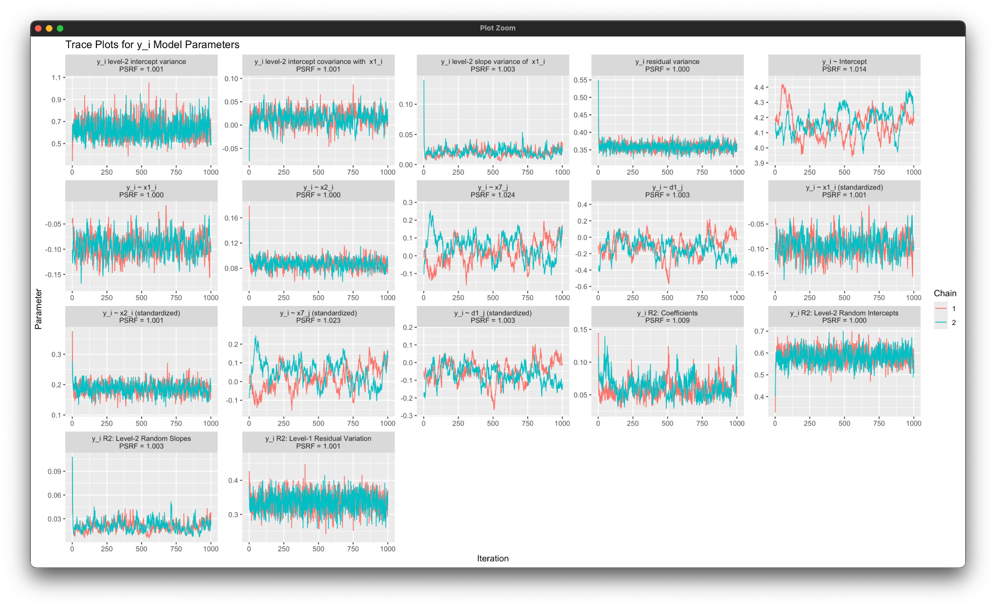
In cases where convergence is not achieved, it is useful to identify which parameter or parameters are responsible. The potential scale reduction factor table indicates that the highest (worst) values prior to convergence are primarily associated with parameter number 8. Listing the optional pinfo keyword on the OPTIONS line prints a table of potential scale reduction factors for all model parameters along with their numeric indices. In some cases (e.g., latent variable models), very high potential scale reduction factors will be associated with standardized regression weights (e.g., due to scaling constraints). In general, these can be ignored, and the focus should be on the unstandardized parameters.
The table for the focal regression model is shown below (unspecified predictor models also have similar tables). The columns of the table give the potential scale reduction factors for the final five checkpoints during the burn-in period. The column labeled [5]contains the diagnostics at the end of the burn-in period). The table indicates that parameter number 8 correspond to the coefficient for a level-2 predictor x3_j.
PARAMETER INFORMATION:

  Printing out Rhat for last 5 comparisons:

  NOTE: Rank-normalized Rhat (Vehtari et al., 2021) is being used.
        This applies rank normalization and chain folding for robust
        convergence detection across all chains.

  Comparing iterations across 4 chains
                  [1]    4001 to 8000
                  [2]    4251 to 8500
                  [3]    4501 to 9000
                  [4]    4751 to 9500
                  [5]    5001 to 10000

                                      [1]    [2]    [3]    [4]    [5]    Prior
Outcome Variable:  y_i

    Variances:
  1  L2 : Var(Intercept)              1.00   1.00   1.00   1.00   1.00   IW(0.0, -3.0)
  2  L2 : Cov(x1_i,Intercept)         1.00   1.00   1.00   1.00   1.00   IW(0.0, -3.0)
  3  L2 : Var(x1_i)                   1.00   1.00   1.01   1.01   1.00   IW(0.0, -3.0)
  4  Residual Var.                    1.00   1.00   1.00   1.00   1.00   IG(-1.0, 0.0)

    Coefficients:
  5  Intercept                        1.02   1.01   1.01   1.01   1.01   N(0.0, Inf)
  6  x1_i                             1.00   1.00   1.00   1.00   1.00   N(0.0, Inf)
  7  x2_i                             1.00   1.00   1.00   1.00   1.00   N(0.0, Inf)
  8  x3_j                             1.02   1.02   1.03   1.03   1.04   N(0.0, Inf)
  9  d_j                              1.01   1.01   1.01   1.01   1.02   N(0.0, Inf)

    Standard Deviations:
 10  L2 : SD(Intercept)               1.00   1.00   1.00   1.00   1.00   ---
 11  L2 : Cor(x1_i,Intercept)         1.00   1.00   1.00   1.00   1.00   ---
 12  L2 : SD(x1_i)                    1.00   1.00   1.01   1.01   1.00   ---
 13  Residual SD                      1.00   1.00   1.00   1.00   1.00   ---

    Standardized Coefficients:
 14  x1_i                             1.00   1.00   1.00   1.00   1.00   ---
 15  x2_i                             1.00   1.00   1.00   1.00   1.00   ---
 16  x3_j                             1.02   1.02   1.03   1.03   1.04   ---
 17  d_j                              1.01   1.01   1.01   1.01   1.02   ---

    Proportion Variance Explained
 18  by Coefficients                  1.01   1.02   1.02   1.02   1.02   ---
 19  by Level-2 Random Intercepts     1.00   1.00   1.00   1.00   1.00   ---
 20  by Level-2 Random Slopes         1.00   1.00   1.01   1.01   1.00   ---
 21  by Level-1 Residual Variation    1.00   1.00   1.00   1.00   1.00   ---
Convergence issues can sometimes be identified by examining trace plots. These are automatically available in the Blimp Studio interface when plotting is enabled in Preferences, and they can be requested in R using rblimp’s trace_plotfunction.
The trace plot of the intercept estimates from the first 5,000 computational cycles is shown below. Plot features such as the number of chains or iterations printed can be set in the Blimp Studio Preferences pull-down menu. Plotting can also be turned off completely in these settings (this can reduce post-processing time considerably).
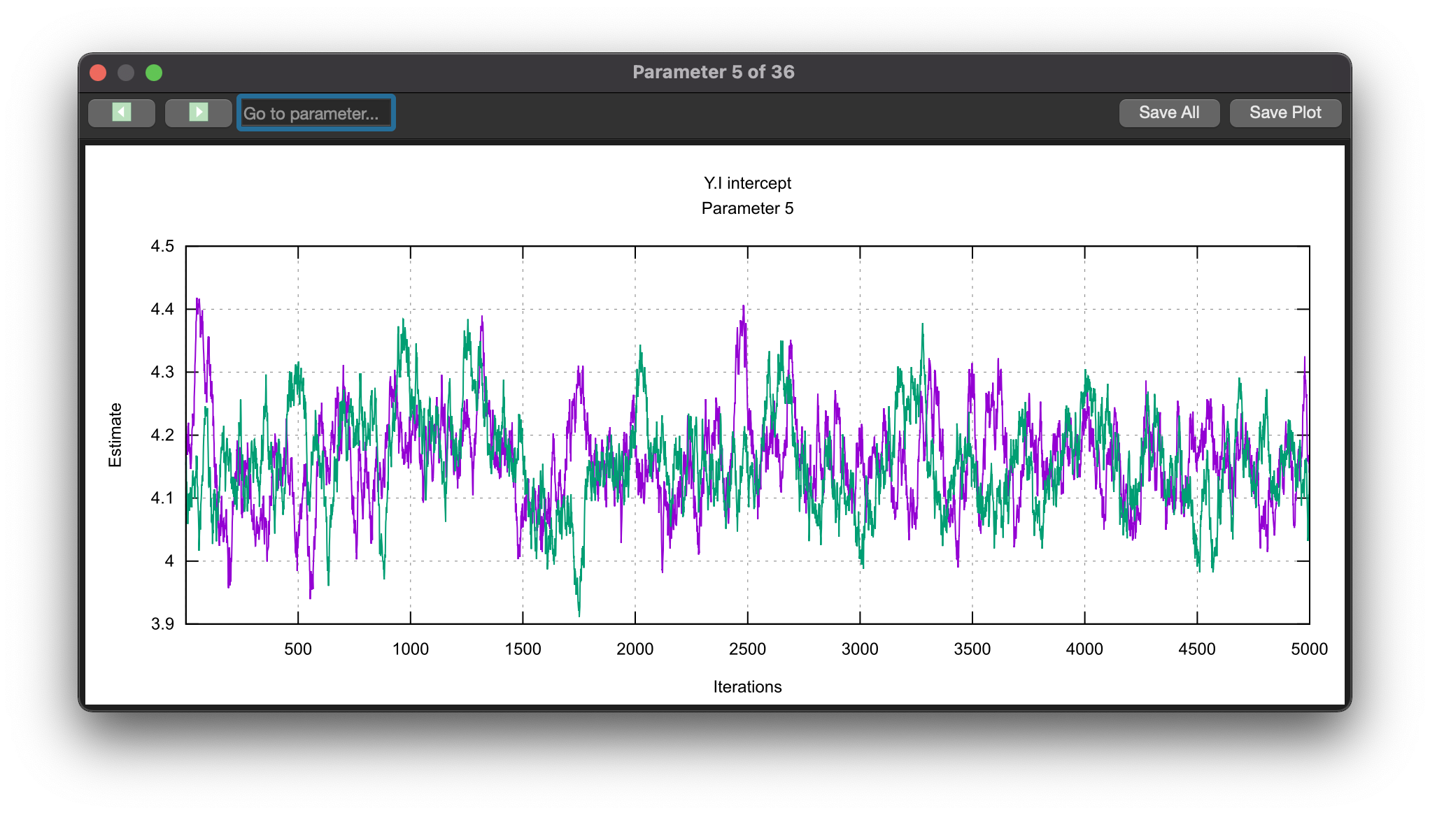
The rblimp script uses the trace_plot function to create comparable graphs. By default, the plotting functions prints the entire burn-in period. The earlier example uses the xlim parameter to restrict plotting to the first 1000 iterations.
Having verified that 10,000 burn-in iterations is sufficient, the next step is to determine whether 10,000 post-burn-in iterations provides sufficiently precise parameter summaries. The parameter summary table for the focal model is shown below.
OUTCOME MODEL ESTIMATES:

  Summaries based on 10000 iterations using 4 chains.
  NOTE: Estimate column based on posterior median.


Outcome Variable:  y_i

Grand Mean Centered: x2_i x3_j
Group Mean Centered: x1_i


Parameters                         Estimate     StdDev       2.5%      97.5%      ChiSq     PValue      N_Eff
                                ------------------------------------------------------------------------------
Variances:
  L2 : Var(Intercept)                 0.620      0.084      0.479      0.809        ---        ---   4032.758
  L2 : Cov(x1_i,Intercept)            0.014      0.016     -0.016      0.047        ---        ---   1706.151
  L2 : Var(x1_i)                      0.020      0.006      0.010      0.034        ---        ---    873.101
  Residual Var.                       0.358      0.011      0.336      0.381        ---        ---   4493.592

Coefficients:
  Intercept                           4.221      0.117      3.984      4.461   1310.057      0.000    112.925
  x1_i                               -0.094      0.019     -0.132     -0.057     24.124      0.000   2155.036
  x2_i                                0.086      0.008      0.070      0.101    121.178      0.000   2669.565
  x3_j                                0.060      0.069     -0.083      0.189      0.716      0.397    153.088
  d_j                                -0.095      0.153     -0.391      0.230      0.371      0.542    154.235

Standard Deviations:
  L2 : SD(Intercept)                  0.787      0.053      0.692      0.899        ---        ---   4054.277
  L2 : Cor(x1_i,Intercept)            0.129      0.137     -0.143      0.391        ---        ---   1749.904
  L2 : SD(x1_i)                       0.140      0.021      0.100      0.184        ---        ---    847.381
  Residual SD                         0.598      0.009      0.580      0.617        ---        ---   4496.283

Standardized Coefficients:
  x1_i                               -0.095      0.019     -0.133     -0.057     23.776      0.000   2196.780
  x2_i                                0.185      0.019      0.149      0.221     98.915      0.000   2418.668
  x3_j                                0.058      0.067     -0.080      0.181      0.724      0.395    152.790
  d_j                                -0.045      0.072     -0.184      0.108      0.378      0.539    154.741

Proportion Variance Explained
  by Coefficients                     0.062      0.017      0.039      0.103        ---        ---    287.912
  by Level-2 Random Intercepts        0.580      0.034      0.513      0.645        ---        ---   2773.153
  by Level-2 Random Slopes            0.020      0.006      0.010      0.034        ---        ---    900.747
  by Level-1 Residual Variation       0.335      0.028      0.280      0.390        ---        ---   1767.491

                                ------------------------------------------------------------------------------
The rightmost column labeled N_Effreports the effective sample size (ESS; Gelman et al., 2014). The ESS gauges whether the post–warm-up parameter summaries have sufficient precision. Numerically, it reflects the effective number of MCMC iterations (the “sample size”) contributing to each summary after accounting for autocorrelation in the MCMC process. Larger values are better, and values above 100 are considered adequate (Gelman et al., 2014, p. 287). Inspecting the N_Eff values across all parameter tables suggests that 10,000 iterations is sufficient because the indices are uniformly large.
When MCMC estimation yields unsatisfactory PSR or ESS values, the first remedy is usually to increase the number of iterations. A practical approach is to raise the values specified on the BURNand ITER lines in increments of 10,000 until the diagnostics fall within acceptable ranges. Although PSR and ESS evaluate different aspects of estimation quality, poor values often occur together, so increasing both settings by the same amount is a straightforward strategy. More persistent estimation problems may indicate that the model is overly complex for the available data, that one or more parameters are not identified by the observed information (e.g., because of problematic missing data patterns), or that the model itself is misspecified. In our experience, models requiring 100,000 to 200,000 iterations often merit closer examination.
Excluding problems arising from coding mistakes or model misspecification, our experience suggests that estimation difficulties most often originate from two sources: sparse incomplete categorical variables with very few observations in one or more categories, and incomplete categorical variables that generate zero cell counts when cross-classified with other categorical variables. Less commonly, convergence problems arise when the model attempts to estimate variability that is effectively absent from the data (e.g., fitting a random coefficient model when slopes do not vary across individuals).
As a practical recommendation, it is wise to inspect the frequency distribution of every categorical variable and examine contingency tables for each pair of discrete variables before fitting a model. Collapsing categories with very small frequencies is often the most effective initial remedy, particularly for multicategorical nominal variables with poorly represented subgroups. Alternatively, manually simplifying the predictor submodel will usually resolve the problem. When convergence difficulties instead reflect overfitting (e.g., estimating random slopes that are effectively fixed), the PSR and ESS diagnostics often help identify the unsupported parameter responsible for the problem. The Blimp YouTube channel has a video dedicated to diagnosing and addressing convergence issues, and that video illustrates how to modify a model to accommodate sparse categorical variables with zero or near-zero cell counts in a contingency table.