6 Multilevel Model Examples
This section illustrates multilevel models in Blimp. In general, it is possible to mix and match features from any examples to create complex analysis models that honor features of the data. Following previous chapters, the examples in this section use a generic notation system where variable names usually consist of an alphanumeric prefix and a numeric suffix (e.g., y, x1, x2, n1, d1, d2). The letter y designates a dependent variable, a d prefix denotes a binary dummy variable, an o prefix indicates an ordinal variable, and an n prefix indicates a multicategorical nominal variable. Additionally, the multilevel examples use a “_i” suffix to denote level-1 variables, “_j” for level-2 variables, and “_k” for level-3 variables (e.g., d_j is a level-2 dummy variable, x_i is a continuous predictor measured at level-1). Blimp determines the levels automatically, so the suffixes are meant as a visual aid for understanding the scripts. Finally, the model equations use “c” and “w” superscripts to indicate grand and group mean centering, respectively. The following list outlines the examples in this section.
6.1: Random Intercept Model
6.2: Two-Level Fully Conditional Specification Multiple Imputation
6.3: Random Coefficient Model
6.4: Multilevel SEM With Random Coefficients
6.5: Alternate Prior Distributions
6:6 Inspecting Residuals
6.7: Heterogeneous Within-Cluster Variances
6.8: Location-Scale Model With Heterogeneous Within-Cluster Variation
6.9: Random Effects Predicting a Level-2 Outcome
6.10: Latent Contextual Effect
6.11: Cross-Level Interaction Effect
6.12: 1-1-1 Mediation With Random Slopes
6.13: 1-1-1 Moderated Mediation
6.14: Within- and Between-Level Mediation
6.15: Two-Level Growth Model
6.16: Three-Level Growth Model
6.17: Three-Level SEM Growth Model
6.18: Two-Level MIMIC Measurement Model
6.19: Sampling Weights
6.20: Partially Nested Designs (Singleton Clusters)
6.21: Discrete-Time Survival Model
6.22: AR(1) Dynamic Structural Equation Model
6.23: VAR(1) Dynamic Structural Equation Model
6.24: Residual (Detrended) Dynamic Structural Equation Model (RDSEM)
6.25: Random Effect Meta Analysis With Known Variances
6.1 Random Intercept Model
This example illustrates a two-level regression model with random intercepts. The regression model is shown below.
\[y_{ij}=\left(\beta_0+b_{0j}\right)+\beta_1x_{1ij}^{c}+\beta_2x_{2ij}^{c}+\beta_3d_{1ij}+\beta_4x_{3j}^{c}+\beta_5d_{2j}+\varepsilon_{ij}\]
The full set of User Guide examples is available from the Examples pull-down menu in the Blimp Studio graphical interface. A GitHub repository with Blimp Studio scripts and data is available here, and a repository containing the rblimp scripts is available here.
The syntax highlights are as follows.
CLUSTERIDcommand identifies a level-2 identifier, automatically inducing random intercepts for all incomplete level-1 variablesORDINALcommand identifies binary predictorsFIXEDcommand defines complete predictorsCENTERcommand applies grand mean centering to predictors- Unspecified associations for predictor variables
DATA: data7.dat;
VARIABLES: level1id level2id v1_i v2_i d1_i v3_i x1_i v4_i
   v5_i x2_i y_i d2_j x3_j v6_j;
CLUSTERID: level2id;
ORDINAL: d1_i d2_j;
MISSING: 999;
FIXED: x2_i d2_j;
CENTER: grandmean = x1_i x2_i x3_j;
MODEL: y_i ~ x1_i x2_i d1_i x3_j d2_j;
SEED: 90291;
BURN: 10000;
ITER: 10000;
The corresponding rblimp script is as follows.
library(rblimp)

mymodel <- rblimp(
  data = data,
  clusterid = 'level2id',
  ordinal = 'd1_i d2_j',
  fixed = 'x2_i d2_j',
  center = 'grandmean = x1_i x2_i x3_j',
  model = 'y_i ~ x1_i x2_i d1_i x3_j d2_j',
  seed = 90291,
  burn = 10000,
  iter = 10000
)

output(mymodel)
posterior_plot(mymodel,'y_i')
6.2 Two-Level Fully Conditional Specification Multiple Imputation
This example illustrates multilevel fully conditional specification multiple imputation as an approach to getting frequentist inference for the analysis from Example 6.1. The analysis model is shown below.
\[y_{ij}=\left(\beta_0+b_{0j}\right)+\beta_1x_{1ij}^{c}+\beta_2x_{2ij}^{c}+\beta_3d_{2ij}+\beta_4x_{3j}^{c}+\beta_5d_{2j}+\varepsilon_{ij}\]
Fully conditional specification should be reserved for random intercept analyses, as applying the procedure to models with random coefficients or interaction terms is known to induce bias (Enders et al., 2020; Grund, Lüdke, & Robitzsch, 2016). Model-based multiple imputation is recommended for such analyses (see Example 6.3).
The full set of User Guide examples is available from the Examples pull-down menu in the Blimp Studio graphical interface. A GitHub repository with Blimp Studio scripts and data is available here, and a repository containing the rblimp scripts is available here.
The syntax highlights are as follows.
CLUSTERIDcommand identifies a level-2 identifier, automatically inducing random intercepts (latent group means) for all level-1 variablesORDINALcommand identifies binary predictorsFIXEDcommand defines complete predictorsFCScommand specifies fully conditional specification multiple imputation with a saturated model at level-1 and level-2 (unstructured within- and between-cluster covariance matrices)FCScommand includes all analysis variablesNIMPScommand specifies 20 imputed data sets (five data sets from each of the default four chains, sampled at equal intervals across the post-burn-in iterations)- Imputations are stacked in a single file with an index variable added in the first column
DATA: data7.dat;
VARIABLES: level1id level2id v1_i v2_i d1_i v3_i x1_i v4_i
   v5_i x2_i y_i d2_j x3_j v6_j;
CLUSTERID: level2id;
ORDINAL: d1_i d2_j;
MISSING: 999;
FIXED: x2_i d2_j;
FCS: y_i x1_i x2_i d1_i x3_j d2_j;
SEED: 90291;
BURN: 10000;
ITER: 10000;
NIMPS: 20;
SAVE: stacked = imps.dat;
Blimp lists the order of the variables in the imputed data sets at the bottom of the output file, and all variables in the input file appear in the output file regardless of whether they were imputed.
VARIABLE ORDER IN IMPUTED DATA:

   stacked = 'imps.dat'

          imp# level1id level2id v1_i v2_i d1_i v3_i x1_i
          v4_i v5_i x2_i y_i d2_j x3_j v6_j
The imputed data sets can be analyzed in other software packages.
R provides an easy platform for analyzing multiple imputations. To illustrate, R script below uses rblimp_fcs to create multiple imputations and the mitml package (Grund, Robitzsch, & Lüdke, 2021) for analysis and pooling. Note that the MISSING and FCS commands are no longer necessary. The former is omitted because that information is contained in the R data file. The FCS command is replaced by a variables parameter that lists the variables to be included in the imputation model. Additionally, the SAVE command is no longer necessary because imputations are automatically stored in an rblimp list object called mymodel@imputations.
library(rblimp)

mymodel <- rblimp_fcs(
  data = data,
  clusterid = 'level2id',
  ordinal = 'd1_i d2_j',
  fixed = 'x2_i d2_j',
  variables = 'y_i x1_i x2_i d1_i x3_j d2_j',
  seed = 90291,
  burn = 10000,
  iter = 10000,
  nimps = 20
)

output(mymodel)

# mitml list
implist <- as.mitml(mymodel)

# analysis and pooling with mitml
results <- with(implist,
   lmer('y_i ~ x1_i + x2_i + d1_i + x3_j + d2_j + (1|level2id)',
   REML = T))
testEstimates(results, extra.pars = T)
6.3 Random Coefficient Model
This example illustrates a two-level regression model with random intercepts and random slopes. The c superscript denotes variables centered at their grand means, and the w (within) superscript denotes variables centered at their level-2 latent group means. The analysis model is shown below.
\[y_{ij}=\left(\beta_0+b_{0j}\right)+\left(\beta_1+b_{1j}\right)x_{1ij}^{w}+\beta_2x_{2ij}^{c}+\beta_3x_{3j}^{c}+\beta_4d_{j}+\varepsilon_{ij}\]
The full set of User Guide examples is available from the Examples pull-down menu in the Blimp Studio graphical interface. A GitHub repository with Blimp Studio scripts and data is available here, and a repository containing the rblimp scripts is available here.
The syntax highlights are as follows.
CLUSTERIDcommand identifies a level-2 identifier, automatically inducing random intercepts for all level-1 variablesORDINALcommand identifies a binary predictorFIXEDcommand identifies complete predictors (optional—speeds computation)CENTERcommand applies grand mean and latent group mean centering to predictorsMODELcommand features a random coefficient listed after the vertical pipe- Unspecified associations for predictor variables
DATA: data8.dat;
VARIABLES: level1id level2id x1_i x2_i y_i v1_i v2_i d_j
   v3_j v4_j v5_j x3_j v6_j v7_j;
CLUSTERID: level2id;
ORDINAL: d_j;
MISSING: 999;
FIXED: d_j;
CENTER: groupmean = x1_i; grandmean = x2_i x3_j;
MODEL: y_i ~ x1_i x2_i x3_j d_j | x1_i;
SEED: 90291;
BURN: 10000;
ITER: 10000;
The corresponding rblimp script is as follows.
library(rblimp)

mymodel <- rblimp(
  data = data,
  clusterid = 'level2id',
  ordinal = 'd_j',
  fixed = 'd_j',
  center = 'groupmean = x1_i; grandmean = x2_i x3_j',
  model = 'y_i ~ x1_i x2_i x3_j d_j | x1_i',
  seed = 90291,
  burn = 10000,
  iter = 10000
)

output(mymodel)
posterior_plot(mymodel,'y_i')
Blimp can save multiple imputations from any model it estimates. Model-based multiple imputations can be saved for a frequentist analysis by adding the SAVE and NIMPS commands. The additional syntax highlights are as follows.
CENTERcommand grand mean centers predictors in the Bayesian output, but saved imputations are on the original metricNIMPScommand specifies 20 imputed data sets (five data sets from each of the default four chains, sampled at equal intervals across the post-burn-in iterations)savelatentkeyword on theOPTIONSline saves the latent group means of the level-1 predictors and the analysis model’s random intercept and random slope residuals- Imputations are stacked in a single file with an index variable added in the first column
DATA: data8.dat;
VARIABLES: level1id level2id x1_i x2_i y_i v1_i v2_i d_j
   v3_j v4_j v5_j x3_j v6_j v7_j;
CLUSTERID: level2id;
ORDINAL: d_j;
MISSING: 999;
FIXED: d_j;
CENTER: groupmean = x1_i; grandmean = x2_i x3_j;
MODEL: y_i ~ x1_i x2_i x3_j d_j | x1_i;
SEED: 90291;
BURN: 10000;
ITER: 10000;
NIMPS: 20;
OPTIONS: savelatent;
SAVE: stacked = imps.dat;
Blimp lists the order of the variables in the imputed data sets at the bottom of the output file, and all variables in the input file appear in the output file regardless of whether they were imputed. The savelatent keyword also saves the latent group means of any level-1 predictors, and these can be used to center variables prior to analyzing the imputations. This example uses x1_i’s latent group means, which are referred to by the name x1_i.mean[level2id].
VARIABLE ORDER IN IMPUTED DATA:

   stacked = 'imps.dat'

     imp# level1id level2id x1_i x2_i y_i v1_i v2_i d_j v3_j
     v4_j v5_j x3_j v6_j v7_j y_i[level2id] y_i$x1_i[level2id]
     x1_i.mean[level2id] x2_i.mean[level2id]
The imputed data sets can be analyzed in other software packages.
R provides an easy platform for analyzing multiple imputations. To illustrate, R script below uses rblimp to create multiple imputations and the mitml package (Grund, Robitzsch, & Lüdke, 2021) for analysis and pooling. Note that the SAVE command and savelatent keyword on the OPTIONS line are no longer necessary because imputations and latent variable scores are automatically stored in an rblimp list object called mymodel@imputations. The pooled estimates are numerically equivalent to the Bayesian results.
library(rblimp)

mymodel <- rblimp(
  data = data,
  clusterid = 'level2id',
  ordinal = 'd_j',
  fixed = 'd_j',
  center = 'groupmean = x1_i; grandmean = x2_i x3_j',
  model = 'y_i ~ x1_i x2_i x3_j d_j | x1_i',
  seed = 90291,
  burn = 10000,
  iter = 10000,
  nimps = 20
)

output(mymodel)
posterior_plot(mymodel,'y_i')

# inspect variable names
names(mymodel)

# mitml list
implist <- as.mitml(mymodel)

# pooled grand means
mean_x2 <- mean(unlist(lapply(implist, function(data) mean(data$x2_i))))
mean_x3 <- mean(unlist(lapply(implist, function(data) mean(data$x3_j))))

# center at imputed latent cluster means
for (i in 1:length(implist)) {
  implist[[i]]$x1cwc_i <- implist[[i]]$x1_i -
  implist[[i]]$"x1_i.mean[level2id]"
}

# analysis and pooling with mitml
results <- with(implist,
  lmer('y_i ~ x1cwc_i + I(x2_i - mean_x2)
   + I(x3_j - mean_x3) + d_j + (1 + x1cwc_i|level2id)',
   REML = T)
)
testEstimates(results, extra.pars = T)
6.4 Multilevel SEM With Random Coefficients
This example illustrates a two-level regression model with random intercepts and random slopes. The c superscript denotes variables centered at their grand means, and the w (within) superscript denotes variables centered at their level-2 latent group means. The analysis model is shown below.
\[y_{ij}=\left(\beta_0+b_{0j}\right)+\left(\beta_1+b_{1j}\right)x_{1ij}^{w}+\beta_2x_{2ij}^{c}+\beta_3x_{3j}^{c}+\beta_4d_{j}+\varepsilon_{ij}\]
The model is cast as a multilevel structural equation model with a pair of normally distributed level-2 latent variables representing the random intercepts and slopes. The level-1 and level-2 models are as follows.
\[y_{ij}=\beta_{0j}+\beta_{1j}x_{1ij}^{w}+\beta_2x_{2ij}^{c}+\varepsilon_{ij}\]
\[\beta_{0j}=\beta_{0}+\beta_3x_{3j}^{c}+\beta_4d_{j}+b_{0j}\]
\[\beta_{1j}=\beta_{1}+b_{1j}\]
The full set of User Guide examples is available from the Examples pull-down menu in the Blimp Studio graphical interface. A GitHub repository with Blimp Studio scripts and data is available here, and a repository containing the rblimp scripts is available here.
The syntax highlights are as follows.
CLUSTERIDcommand identifies level-2 and level-3 identifiers (order doesn’t matter), automatically inducing random intercepts for all level-1 and level-2 variablesORDINALcommand identifies binary predictorsFIXEDcommand defines complete predictorsCENTERcommand applies grand mean and latent group mean centering to predictorsLATENTcommand defines two between-cluster latent variables representing the random intercepts and slopesMODELcommand uses labels ending in a colon to group models and order their summary tables on the outputMODELcommand estimates the random intercept and slope meansMODELcommand sets the intercept of the regression equation equal to the level-2 latent mean (i.e.,1@beta0_j)MODELcommand omits the random coefficient listed after the vertical pipeMODELcommand sets the random predictor’s slope equal to the random coefficient (i.e.,x1_i@beta1_j)MODELcommand specifies correlation between random intercepts and random slopes (level-2 latent variables)
DATA: data8.dat;
VARIABLES: level1id level2id x1_i x2_i y_i v1_i v2_i d_j
   v3_j v4_j v5_j x3_j v6_j v7_j;
CLUSTERID: level2id;
ORDINAL: d_j;
MISSING: 999;
LATENT: level2id = beta0_j beta1_j;
FIXED: d_j;
CENTER: groupmean = x1_i; grandmean = x2_i x3_j;
MODEL:
  level2.model:
  beta0_j ~ 1 x3_j d_j;
  beta1_j ~ 1;
  beta0_j ~~ beta1_j;
  level1.model:
  y_i ~ 1@beta0_j x1_i@beta1_j x2_i;
SEED: 90291;
BURN: 10000;
ITER: 10000;
The corresponding rblimp script is as follows.
library(rblimp)
mymodel <- rblimp(
  data = data,
  clusterid = 'level2id',
  ordinal = 'd_j',
  latent = 'level2id = beta0_j beta1_j',
  fixed = 'd_j',
  center = 'groupmean = x1_i; grandmean = x2_i x3_j',
  model = '
    level2.model:
    beta0_j ~ 1 x3_j d_j;
    beta1_j ~ 1;
    beta0_j ~~ beta1_j;
    level1.model:
    y_i ~ 1@beta0_j x1_i@beta1_j x2_i',
  seed = 90291,
  burn = 10000,
  iter = 10000
)

output(mymodel)
The random effect parameter estimates no longer appear on the same table when using the multilevel SEM specification. Rather, each equation has its own summary table. For example, the latent variable summary tables are shown below.
Latent Variable:   beta0_j

Grand Mean Centered: x3_j


Parameters                         Estimate     StdDev       2.5%      97.5%      ChiSq     PValue      N_Eff
                                ------------------------------------------------------------------------------
Variances:
  Residual Var.                       0.619      0.085      0.482      0.817        ---        ---   7393.214

Coefficients:
  Intercept                           4.211      0.107      4.002      4.425   1541.547      0.000   7803.019
  x3_j                                0.050      0.069     -0.086      0.186      0.520      0.471   8208.559
  d_j                                -0.077      0.141     -0.360      0.195      0.307      0.579   8722.335

Standard Deviations:
  Residual SD                         0.787      0.053      0.694      0.904        ---        ---   7413.153

Standardized Coefficients:
  x3_j                                0.065      0.088     -0.109      0.235      0.530      0.467   8261.885
  d_j                                -0.048      0.086     -0.218      0.120      0.312      0.576   8755.233

Proportion Variance Explained
  by Coefficients                     0.016      0.020      0.001      0.075        ---        ---   9207.095
  by Residual Variation               0.984      0.020      0.925      0.999        ---        ---   9207.095

                                ------------------------------------------------------------------------------


Latent Variable:   beta1_j

Parameters                         Estimate     StdDev       2.5%      97.5%      ChiSq     PValue      N_Eff
                                ------------------------------------------------------------------------------
Variances:
  Residual Var.                       0.020      0.006      0.011      0.033        ---        ---   1022.862

Coefficients:
  Intercept                          -0.094      0.019     -0.132     -0.056     23.228      0.000   1823.284

Standard Deviations:
  Residual SD                         0.141      0.020      0.103      0.183        ---        ---    990.542

Proportion Variance Explained
  by Coefficients                     0.000      0.000      0.000      0.000        ---        ---        ---
  by Residual Variation               1.000      0.000      1.000      1.000        ---        ---        ---

                                ------------------------------------------------------------------------------


Covariance Matrix: beta0_j beta1_j

Parameters                         Estimate     StdDev       2.5%      97.5%      ChiSq     PValue      N_Eff
                                ------------------------------------------------------------------------------
Covariances:
  Cov(beta0_j,beta1_j)                0.013      0.016     -0.017      0.047      0.722      0.396   2148.438

Correlations:
  Cor(beta0_j,beta1_j)                0.122      0.139     -0.157      0.385      0.760      0.383   2075.986

                                ------------------------------------------------------------------------------
6.5 Alternate Prior Distributions for Random Effect Covariance Matrix
This example illustrates how to examine the influence of different prior distributions on the level-2 covariance matrix of the random effects. The analysis model is the following two-level regression with random intercepts and random slopes. The c superscript denotes variables centered at their grand means, and the w (within) superscript denotes variables centered at their level-2 latent group means.
\[y_{ij}=\left(\beta_0+b_{0j}\right)+\left(\beta_1+b_{1j}\right)x_{1ij}^{w}+\beta_2x_{2ij}^{c}+\varepsilon_{ij}\]
The between-cluster covariance matrix of the random effects is a 2 by 2 matrix in this example. Blimp offers three “off-the-shelf” inverse Wishart priors for the covariance matrix, and it is also possible to use a so-called separation strategy that applies distinct priors to variances and the intercept-slope correlation.
Considering the inverse Wishart options, the default prior2 setting is less informative because it subtracts the number of dimensions plus 1 from the degrees of freedom, and it adds nothing to the sum of squares and cross-products; prior1 is more informative because it adds the number of dimensions plus 1 to the degrees of freedom, and it adds an identity matrix to the sum of squares and cross-products; prior3 adds zero degrees of freedom and adds zero to the sums of squares.
The full set of User Guide examples is available from the Examples pull-down menu in the Blimp Studio graphical interface. A GitHub repository with Blimp Studio scripts and data is available here, and a repository containing the rblimp scripts is available here.
The code block below shows the default specification, the syntax highlights for which are as follows.
CLUSTERIDcommand identifies a level-2 identifier, automatically inducing random intercepts for all level-1 variablesCENTERcommand applies grand mean and latent group mean centeringMODELcommand features a random coefficient listed after the vertical pipe- Unspecified associations for predictor variables
prior2keyword on theOPTIONSline (optional) specifies the default inverse Wishart prior
DATA: data8.dat;
VARIABLES: level1id level2id x1_i x2_i y_i v1_i v2_i d_j
   v3_j v4_j v5_j x3_j v6_j v7_j;
CLUSTERID: level2id;
MISSING: 999;
CENTER: groupmean = x1_i; grandmean = x2_i;
MODEL: y_i ~ x1_i x2_i | x1_i;
SEED: 90291;
BURN: 10000;
ITER: 10000;
OPTIONS: prior2;
The corresponding rblimp script is as follows.
library(rblimp)

mymodel <- rblimp(
  data = data,
  clusterid = 'level2id',
  center = 'groupmean = x1_i;
  grandmean = x2_i',
  model = 'y_i ~ x1_i x2_i | x1_i',
  seed = 90291,
  burn = 10000,
  iter = 10000,
  options = 'prior2'
)

output(mymodel)
posterior_plot(mymodel,'y_i')
Similarly, the code block below shows the specification for the more informative prior1 inverse Wishart option.
DATA: data8.dat;
VARIABLES: level1id level2id x1_i x2_i y_i v1_i v2_i d_j
   v3_j v4_j v5_j x3_j v6_j v7_j;
CLUSTERID: level2id;
MISSING: 999;
CENTER: groupmean = x1_i; grandmean = x2_i;
MODEL: y_i ~ x1_i x2_i | x1_i;
SEED: 90291;
BURN: 10000;
ITER: 10000;
OPTIONS: prior1;
The corresponding rblimp script is as follows.
library(rblimp)

mymodel <- rblimp(
  data = data,
  clusterid = 'level2id',
  center = 'groupmean = x1_i;
  grandmean = x2_i',
  model = 'y_i ~ x1_i x2_i | x1_i',
  seed = 90291,
  burn = 10000,
  iter = 10000,
  options = 'prior1'
)

output(mymodel)
posterior_plot(mymodel,'y_i')
Comparing the magnitude of the point estimates provides a gauge about the prior distribution’s impact. The output table for the default prior2 specification is shown immediately below, and the second output table shows the results from the more informative prior1 specification.
Outcome Variable:  y_i

Grand Mean Centered: x2_i
Group Mean Centered: x1_i


Parameters                         Estimate     StdDev       2.5%      97.5%      ChiSq     PValue      N_Eff
                                ------------------------------------------------------------------------------
Variances:
  L2 : Var(Intercept)                 0.616      0.083      0.479      0.803        ---        ---   7045.482
  L2 : Cov(x1_i,Intercept)            0.016      0.016     -0.014      0.048        ---        ---   2303.478
  L2 : Var(x1_i)                      0.020      0.006      0.011      0.034        ---        ---    884.999
  Residual Var.                       0.358      0.011      0.337      0.381        ---        ---   4967.417

Coefficients:
  Intercept                           4.172      0.070      4.036      4.309   3602.505      0.000    105.075
  x1_i                               -0.094      0.019     -0.132     -0.055     23.132      0.000   1473.592
  x2_i                                0.087      0.008      0.071      0.102    118.636      0.000   2253.065

Standard Deviations:
  L2 : SD(Intercept)                  0.785      0.052      0.692      0.896        ---        ---   7063.588
  L2 : Cor(x1_i,Intercept)            0.145      0.134     -0.125      0.395        ---        ---   2244.711
  L2 : SD(x1_i)                       0.141      0.021      0.103      0.184        ---        ---    842.657
  Residual SD                         0.598      0.009      0.581      0.617        ---        ---   4970.641

Standardized Coefficients:
  x1_i                               -0.095      0.020     -0.134     -0.055     22.818      0.000   1547.738
  x2_i                                0.188      0.019      0.152      0.225    100.677      0.000   2352.504

Proportion Variance Explained
  by Coefficients                     0.047      0.009      0.033      0.066        ---        ---   2335.194
  by Level-2 Random Intercepts        0.589      0.033      0.524      0.653        ---        ---   6218.012
  by Level-2 Random Slopes            0.021      0.006      0.011      0.035        ---        ---    917.893
  by Level-1 Residual Variation       0.342      0.027      0.289      0.396        ---        ---   6661.272

                                ------------------------------------------------------------------------------
Outcome Variable: y_i
Grand Mean Centered: x2_i
Group Mean Centered: x1_i
Parameters Estimate StdDev 2.5% 97.5% ChiSq PValue N_Eff
------------------------------------------------------------------------------
Variances:
L2 : Var(Intercept) 0.592 0.078 0.464 0.765 --- --- 7054.570
L2 : Cov(x1_i,Intercept) 0.017 0.018 -0.017 0.054 --- --- 3358.916
L2 : Var(x1_i) 0.039 0.007 0.028 0.056 --- --- 2091.426
Residual Var. 0.355 0.011 0.333 0.378 --- --- 6035.156
Coefficients:
Intercept 4.171 0.071 4.029 4.314 3441.313 0.000 100.629
x1_i -0.093 0.023 -0.138 -0.048 16.027 0.000 1348.531
x2_i 0.087 0.008 0.071 0.102 120.009 0.000 2416.956
Standard Deviations:
L2 : SD(Intercept) 0.769 0.050 0.681 0.875 --- --- 6994.811
L2 : Cor(x1_i,Intercept) 0.112 0.112 -0.110 0.326 --- --- 3334.520
L2 : SD(x1_i) 0.198 0.018 0.167 0.237 --- --- 2055.447
Residual SD 0.596 0.009 0.577 0.614 --- --- 6033.274
Standardized Coefficients:
x1_i -0.095 0.024 -0.141 -0.048 15.883 0.000 1370.382
x2_i 0.188 0.019 0.153 0.226 100.721 0.000 2495.315
Proportion Variance Explained
by Coefficients 0.048 0.009 0.032 0.068 --- --- 2011.718
by Level-2 Random Intercepts 0.569 0.033 0.504 0.634 --- --- 5879.620
by Level-2 Random Slopes 0.041 0.008 0.028 0.059 --- --- 2388.730
by Level-1 Residual Variation 0.341 0.026 0.290 0.392 --- --- 7301.515
------------------------------------------------------------------------------The default prior 2’s random slope variance is roughly half as large as that of the more informative prior (0.020 vs. 0.039), and the two estimates differed by about 2.7 posterior standard deviation units (a very large difference). As a proportion of the total variance, the R2 effect sizes attributable to the random slopes (Rights & Sterba, 2019) were also quite different (2.1% vs. 4.1%).
The separation strategy (Barnard, McCulloch, & Meng, 2000; Liu, Zhang, & Grimm, 2016) assigns distinct priors to the diagonal and off-diagonal elements of the covariance matrix. An analogous strategy can be implemented in Blimp by specifying the random intercepts and slopes as a pair of level-2 latent variables. The focal model is cast as a multilevel structural equation model with a pair of normally distributed level-2 latent variables representing the random intercepts and slopes. The focal model features these latent variables as predictors, as shown below.
\[\beta_{0j}=\beta_{0}+b_{0j}\]
\[\beta_{1j}=\beta_{1}+b_{1j}\]
\[y_{ij}=\beta_{0j}+\beta_{1j}x_{1ij}^{w}+\beta_2x_{2ij}^{c}+\varepsilon_{ij}\]
Note that the coefficient of the random slope predictor is implicitly fixed to one in this specification.
This specification assigns separate inverse gamma priors to the random intercept and slope variances, and it specifies a beta prior distribution to their correlation. Blimp uses a multilevel extension of the procedure described in Merkle and Rosseel (2018). Computer simulation studies suggest that the separation strategy gives more accurate estimates of the variance components, although the correlation estimate may be attenuated when the number of level-2 units is small (Keller & Enders, 2021). The unique syntax highlights for the code block are as follows.
LATENTcommand defines two between-cluster latent variables representing the random intercepts and slopesMODELcommand uses labels ending in a colon to group models and order their summary tables on the outputMODELcommand estimates the random intercept and slope meansMODELcommand sets the intercept of the regression equation equal to the level-2 latent mean (1@beta0.j)MODELcommand omits the random coefficient listed after the vertical pipeMODELcommand sets the random predictor’s slope equal to the random coefficient (x1_i@beta1_j)MODELcommand specifies correlation between random intercepts and random slopes (level-2 latent variables)OPTIONScommand lists the use_phantom keyword to invoke a phantom variable specification that assigns distinct priors to latent variable variances and their correlation
DATA: data8.dat;
VARIABLES: level1id level2id x1_i x2_i y_i v1_i v2_i d_j
   v3_j v4_j v5_j x3_j v6_j v7_j;
CLUSTERID: level2id;
MISSING: 999;
LATENT: level2id = beta0_j beta1_j;
CENTER: groupmean = x1_i; grandmean = x2_i;
MODEL:
  latent.variables:
  beta0_j ~ 1;
  beta1_j ~ 1;
  beta0_j ~~ beta1_j;
  focal.model:
  y_i ~ 1@beta0_j x1_i@beta1_j x2_i;
SEED: 90291;
BURN: 10000;
ITER: 10000;
OPTIONS: use_phantom;
The corresponding rblimp script is as follows.
library(rblimp)

mymodel <- rblimp(
  data = data,
  clusterid = 'level2id',
  latent = 'level2id = beta0_j beta1_j',
  center = 'groupmean = x1_i;
  grandmean = x2_i',
  model = '
    latent.variables:
    beta1_j ~ 1;
    beta0_j ~~ beta1_j;
    focal.model:
    y_i ~ 1@beta0_j x1_i@beta1_j x2_i',
  seed = 90291,
  burn = 10000,
  iter = 10000,
  options = 'use_phantom'
)
output(mymodel)
posterior_plot(mymodel)
The random effect parameter estimates no longer appear on the same table when employing the separation strategy because the random intercepts and slopes are latent variables with their own equations and summary tables. The analysis model table shows the random intercept variance, and the level-2 latent variable’s (random slope) variance and correlation appear in separate tables.
Latent Variable:   beta0_j

Parameters                         Estimate     StdDev       2.5%      97.5%      ChiSq     PValue      N_Eff
                                ------------------------------------------------------------------------------
Variances:
  Residual Var.                       0.604      0.081      0.470      0.790        ---        ---   7066.012

Coefficients:
  Intercept                           4.169      0.071      4.032      4.309   3463.979      0.000   5780.931

Standard Deviations:
  Residual SD                         0.777      0.051      0.686      0.889        ---        ---   7023.788

Proportion Variance Explained
  by Coefficients                     0.000      0.000      0.000      0.000        ---        ---        ---
  by Residual Variation               1.000      0.000      1.000      1.000        ---        ---        ---

                                ------------------------------------------------------------------------------


Latent Variable:   beta1_j

Parameters                         Estimate     StdDev       2.5%      97.5%      ChiSq     PValue      N_Eff
                                ------------------------------------------------------------------------------
Variances:
  Residual Var.                       0.019      0.005      0.011      0.032        ---        ---    635.014

Coefficients:
  Intercept                          -0.094      0.019     -0.132     -0.057     24.396      0.000   1837.969

Standard Deviations:
  Residual SD                         0.137      0.019      0.103      0.178        ---        ---    618.267

Proportion Variance Explained
  by Coefficients                     0.000      0.000      0.000      0.000        ---        ---        ---
  by Residual Variation               1.000      0.000      1.000      1.000        ---        ---        ---

                                ------------------------------------------------------------------------------


Phantom Variable Correlations:

Parameters                         Estimate     StdDev       2.5%      97.5%      ChiSq     PValue      N_Eff
                                ------------------------------------------------------------------------------

  beta0_j <-> beta1_j                 0.091      0.131     -0.148      0.353        ---        ---     48.030

                                ------------------------------------------------------------------------------
6.6 Inspecting Residuals
This example illustrates how to inspect the level-1 and level-2 residuals (random effects) from a two-level regression model with random intercepts and random slopes. The analysis model, shown below, is the same as the one from Example 6.4. The c superscript denotes variables centered at their grand means, and the w (within) superscript denotes variables centered at their level-2 latent group means.
\[y_{ij}=\left(\beta_0+b_{0j}\right)+\left(\beta_1+b_{1j}\right)x_{1ij}^{w}+\beta_2x_{2ij}^{c}+\varepsilon_{ij}\]
The full set of User Guide examples is available from the Examples pull-down menu in the Blimp Studio graphical interface. A GitHub repository with Blimp Studio scripts and data is available here, and a repository containing the rblimp scripts is available here.
The syntax highlights are as follows.
CLUSTERIDcommand identifies a level-2 identifier, automatically inducing random intercepts for all level-1 variablesCENTERcommand applies grand mean and latent group mean centering to predictors in the Bayesian output, but saved imputations are on the original metricMODELcommand features a random coefficient listed after the vertical pipe- Unspecified associations for predictor variables
savelatentkeyword on theOPTIONSline saves the latent group means of the level-1 predictors and the analysis model’s random intercept and random slope residualssaveresidualkeyword on theOPTIONSline saves level-1 residualsNIMPScommand specifies 20 imputed data sets (five data sets from each of the default four chains, sampled at equal intervals across the post-burn-in iterations)- Imputations are stacked in a single file with an index variable added in the first column
DATA: data8.dat;
VARIABLES: level1id level2id x1_i x2_i y_i v1_i v2_i d_j
  v3_j v4_j v5_j x3_j v6_j v7_j;
CLUSTERID: level2id;
MISSING: 999;
CENTER: groupmean = x1_i; grandmean = x2_i;
MODEL: y_i ~ x1_i x2_i | x1_i;
SEED: 90291;
BURN: 10000;
ITER: 10000;
NIMPS: 20;
OPTIONS: savelatent saveresidual;
SAVE: stacked = imps.dat;
Blimp lists the order of the variables in the imputed data sets at the bottom of the output file, and all variables in the input file appear in the output file regardless of whether they were imputed. The latent group means, random effects, and level-1 residuals are appended to the end of the file. Latent group means are designated by appending the level-2 identifier in square brackets to the end of a predictor variable’s name (e.g., x1_i.mean[level2id] and x2_i_mean[level2id]). The analysis model’s random intercepts are denoted by appending the level-2 identifier in square brackets to the end of an outcome variable’s name (e.g., y_i[level2id]). Random slope residuals are indicated by joining the outcome and random predictor variables with a $ sign (e.g., y_i$x1_i[level2id]). Finally, level-1 residuals are indicated by appending .residual to the end of the outcome variable’s name (e.g., y_i.residual).
VARIABLE ORDER IN IMPUTED DATA:

   stacked = 'imps.dat'

    imp# level1id level2id x1_i x2_i y_i v1_i v2_i d_j v3_j
    v4_j v5_j x3_j v6_j v7_j y_i[level2id] y_i$x1_i[level2id]
    x1_i.mean[level2id] x2_i.mean[level2id] y_i.residual
The imputed data sets can be analyzed in other software packages.
R provides an easy platform for analyzing multiple imputations. To illustrate, R script below uses rblimp to create multiple imputations for graphing. Note that the SAVE command and savelatent keyword on the OPTIONS line are no longer necessary because imputations and latent variable scores are automatically stored in an rblimp list object called mymodel@imputations.
library(rblimp)

mymodel <- rblimp(
  data = data,
  clusterid = 'level2id',
  ordinal = 'd_j',
  fixed = 'd_j',
  center = 'groupmean = x1_i; grandmean = x2_i x3_j',
  model = 'y_i ~ x1_i x2_i x3_j d_j | x1_i',
  seed = 90291,
  burn = 10000,
  iter = 10000,
  nimps = 20
)
output(mymodel)
posterior_plot(mymodel)

# inspect variable names in imputed data
names(mymodel)

# unlist imputed data sets into a stacked file
dat2plot <- do.call(rbind, mymodel@imputations)
# plot level-1 residuals
hist(dat2plot$y_i.residual,breaks = 50)
# plot random intercepts
hist(dat2plot$"y_i[level2id]",breaks = 50)
# plot random slopes
hist(dat2plot$"y_i$x1_i[level2id]",breaks = 50)
6.7 Heterogeneous Within-Cluster Variation
This example illustrates a two-level regression model with random intercepts and slopes and heterogeneous within-cluster variances. The analysis model below is the same one as Example 6.3, but the variance of the within-cluster residuals differs across clusters. The c superscript denotes variables centered at their grand means, and the w (within) superscript denotes variables centered at their level-2 latent group means.
\[y_{ij}=\left(\beta_0+b_{0j}\right)+\left(\beta_1+b_{1j}\right)x_{1ij}^{w}+\beta_2x_{2ij}^{c}+\beta_3x_{3j}^{c}+\beta_4d_{j}+\varepsilon_{ij}\]
Blimp provides two methods for modeling heterogeneous within-cluster variation. The first is an approach described by Kasim and Raudenbush (1998). Their model views cluster-specific variances as a level-2 variable. Unlike the location-scale model in Example 6.8, the Kasim and Raudenbush method does not allow random variation to correlate with or link to other level-2 variables and random effects. Thus, the intent of this model is to simply adjust for heteroscedasticity in the same spirit as robust standard errors.
The full set of User Guide examples is available from the Examples pull-down menu in the Blimp Studio graphical interface. A GitHub repository with Blimp Studio scripts and data is available here, and a repository containing the rblimp scripts is available here.
The code block below shows the setup for the Kasim and Raudenbush (1998) approach to modeling heterogeneous variation. The syntax highlights are listed below.
CLUSTERIDcommand identifies a level-2 identifier, automatically inducing random intercepts for all level-1 variablesORDINALcommand identifies a binary predictorFIXEDcommand identifies complete predictors (optional—speeds computation)CENTERcommand applies grand mean and latent group mean centering to predictorsMODELcommand features a random coefficient listed after the vertical pipe- Unspecified associations for predictor variables
hevkeyword onOPTIONSline specifies heterogeneous within-cluster variances (Kasim & Raudenbush, 1998)
DATA: data8.dat;
VARIABLES: level1id level2id x1_i x2_i y_i v1_i v2_i d_j
   v3_j v4_j v5_j x3_j v6_j v7_j;
CLUSTERID: level2id;
ORDINAL: d_j;
MISSING: 999;
FIXED: d_j;
CENTER: groupmean = x1_i; grandmean = x2_i x3_j;
MODEL: y_i ~ x1_i x2_i x3_j d_j | x1_i;
SEED: 90291;
BURN: 10000;
ITER: 10000;
OPTIONS: hev;
The corresponding rblimp script is as follows.
library(rblimp)

mymodel <- rblimp(
  data = data,
  clusterid = 'level2id',
  ordinal = 'd_j',
  fixed = 'd_j',
  center = 'groupmean = x1_i; grandmean = x2_i x3_j',
  model = 'y_i ~ x1_i x2_i x3_j d_j | x1_i',
  seed = 90291,
  burn = 10000,
  iter = 10000,
  options = 'hev'
)

output(mymodel)
posterior_plot(mymodel,'y_i')
MCMC estimation yields an estimate of the variation within each cluster. To convey the magnitude of the variational differences, Blimp computes the mean and quartiles of the variance distribution and includes these summaries on the output. The output excerpt below shows part of the main summary table from the example.
OUTCOME MODEL ESTIMATES:

  Summaries based on 10000 iterations using 2 chains.
  NOTE: Estimate column based on posterior median.

Outcome Variable:  y_i

Grand Mean Centered: x2_i x3_j
Group Mean Centered: x1_i

Parameters                         Estimate     StdDev       2.5%      97.5%      ChiSq     PValue      N_Eff
                                ------------------------------------------------------------------------------
Variances:
  L2 : Var(Intercept)                 0.648      0.088      0.507      0.851        ---        ---   2275.976
  L2 : Cov(x1_i,Intercept)            0.026      0.014     -0.000      0.056        ---        ---   1353.623
  L2 : Var(x1_i)                      0.014      0.006      0.006      0.028        ---        ---    399.327
  Heterogeneity Index                 0.207      0.036      0.149      0.288        ---        ---   2690.785
  Q25% Residual Var.                  0.188      0.011      0.168      0.211        ---        ---   3546.726
  Q50% Residual Var.                  0.296      0.016      0.267      0.328        ---        ---   4939.882
  Mean Residual Var.                  0.373      0.016      0.345      0.406        ---        ---   2717.476
  Q75% Residual Var.                  0.476      0.028      0.426      0.534        ---        ---   4386.602

Coefficients:
  Intercept                           4.052      0.066      3.920      4.176   3817.062      0.000    138.824
  x1_i                               -0.100      0.018     -0.136     -0.065     31.811      0.000   2253.634
  x2_i                                0.084      0.007      0.070      0.098    134.698      0.000   2252.413
  x3_j                                0.001      0.066     -0.129      0.130      0.001      0.977    165.748
  d_j                                -0.133      0.131     -0.387      0.114      0.992      0.319    149.737

Standard Deviations:
  L2 : SD(Intercept)                  0.805      0.054      0.712      0.923        ---        ---   2313.479
  L2 : Cor(x1_i,Intercept)            0.276      0.137     -0.002      0.527        ---        ---    873.125
  L2 : SD(x1_i)                       0.120      0.023      0.078      0.167        ---        ---    375.488

Standardized Coefficients:
  x1_i                               -0.099      0.018     -0.134     -0.065     31.210      0.000   2468.622
  x2_i                                0.177      0.017      0.145      0.211    107.894      0.000   1829.521
  x3_j                                0.001      0.063     -0.122      0.124      0.001      0.976    166.801
  d_j                                -0.063      0.061     -0.180      0.054      1.008      0.315    150.247

Proportion Variance Explained
  by Coefficients                     0.053      0.012      0.036      0.085        ---        ---    296.544
  by Level-2 Random Intercepts        0.590      0.034      0.525      0.656        ---        ---   2054.919
  by Level-2 Random Slopes            0.014      0.006      0.006      0.027        ---        ---    408.040
  by Level-1 Residual Variation       0.225      0.024      0.181      0.275        ---        ---   2562.876

                                ------------------------------------------------------------------------------
6.8 Location–Scale Model With Heterogeneous Within-Cluster Variation
This example illustrates a two-level location-scale model with random intercepts, random slopes, and random heterogeneous within-cluster variances. Hedeker, Mermelstein, and Demirtas (2008) and more recently McNeish (2021) describe the model in detail. The analysis model below is the same one as Example 6.4, but the variance of the within-cluster residuals differs across clusters. The c superscript denotes variables centered at their grand means, and the w (within) superscript denotes variables centered at their level-2 latent group means.
\[y_{ij}=\left(\beta_0+b_{0j}\right)+\left(\beta_1+b_{1j}\right)x_{1ij}^{w}+\beta_2x_{2ij}^{c}+\beta_3x_{3j}^{c}+\beta_4d_{j}+\varepsilon_{ij}\]
Following Example 6.4, the model is cast as a multilevel structural equation model with a pair of normally distributed level-2 latent variables representing the random intercepts and slopes. The level-1 and level-2 models are as follows.
\[y_{ij}=\beta_{0j}+\beta_{1j}x_{1ij}^{w}+\beta_2x_{2ij}^{c}+\varepsilon_{ij}\]
\[\beta_{0j}=\beta_{0}+\beta_3x_{3j}^{c}+\beta_4d_{j}+b_{0j}\]
\[\beta_{1j}=\beta_{1}+b_{1j}\]
A location-scale model expresses the natural log of the within-cluster variance as a level-2 latent variable (random effect). The mean and variance of this latent variable encode the typical amount of variation and between-cluster differences in the within-cluster variation (on the logarithmic metric). The scale model has both a within-cluster and between-cluster component, and predictors can be added at each level. The equations below add a predictor at each level.
\[\gamma_{0j}=\gamma_{0}+\gamma_2d_{j}+g_{0j}\]
\[\operatorname{ln}(\sigma_{\varepsilon_{ij}}^2)=\gamma_{0j}+\gamma_1x_{1ij}^{w}\]
This approach allows within-cluster variation to function as both an outcome and a predictor of distal level-2 outcomes, and it could also function as a moderator. It is typical to allow the logarithmic latent variable to correlate with the random intercepts and slopes from the focal model. The code block below shows the basic setup for a location-scale model where observation-level variation is a function of a level-1 and level-2 predictor and a level-2 random effect.
The full set of User Guide examples is available from the Examples pull-down menu in the Blimp Studio graphical interface. A GitHub repository with Blimp Studio scripts and data is available here, and a repository containing the rblimp scripts is available here.
The syntax highlights are listed below.
CLUSTERIDcommand identifies a level-2 identifier, automatically inducing random intercepts for all level-1 variablesORDINALcommand identifies a binary predictorFIXEDcommand defines a complete predictorLATENTcommand initializes three level-2 latent variables that represent the random intercepts, random slopes, and random within-cluster variances on the logarithmic scaleCENTERcommand applies grand mean and latent group mean centering to predictorsMODELcommand uses labels ending in a colon to group models and order their summary tables on the outputMODELcommand estimates the latent variable meansMODELcommand sets the intercept of the regression equation equal to the level-2 latent mean (1@beta0_j)MODELcommand omits the random coefficient listed after the vertical pipeMODELcommand sets the random predictor’s slope equal to the random coefficient (x1_i@beta1_j)MODELcommand includes a variance model for the outcome using thevar(y1_i)functionMODELcommand sets the intercept of the log-variance model equal to the level-2 latent mean (e.g.,var(y1_i) ~ 1@logvar_j)MODELcommand specifies correlations among all random effects
DATA: data8.dat;
VARIABLES: level1id level2id x1_i x2_i y_i v1_i v2_i d_j
   v3_j v4_j v5_j x3_j v6_j v7_j;
CLUSTERID: level2id;
ORDINAL: d_j;
MISSING: 999;
LATENT: level2id = beta0_j beta1_j logvar_j;
FIXED: d_j;
CENTER: groupmean = x1_i; grandmean = x2_i x3_j;
MODEL:
  level2.model:
  beta0_j ~ 1 x3_j d_j;
  beta1_j ~ 1;
  beta0_j ~~ beta1_j;
  level1.model:
  y_i ~ 1@beta0_j x1_i@beta1_j x2_i;
  variance.model:
  logvar_j ~ 1 d_j;
  var(y_i) ~ 1@logvar_j x1_i;
  logvar_j ~~ beta0_j beta1_j;
SEED: 90291;
BURN: 10000;
ITER: 10000;
The corresponding rblimp script is as follows.
library(rblimp)

mymodel <- rblimp(
  data = data,
  clusterid = 'level2id',
  ordinal = 'd_j',
  latent = 'level2id = beta0_j beta1_j logvar_j',
  fixed = 'd_j',
  center = 'groupmean = x1_i; grandmean = x2_i x3_j',
  model = '
    level2.model:
    beta0_j ~ 1 x3_j d_j;
    beta1_j ~ 1;
    beta0_j ~~ beta1_j;
    level1.model:
    y_i ~ 1@beta0_j x1_i@beta1_j x2_i;
    variance.model:
    logvar_j ~ 1 d_j;
    var(y_i) ~ 1@logvar_j x1_i;
    logvar_j ~~ beta0_j beta1_j',
  seed = 90291,
  burn = 10000,
  iter = 10000
)

output(mymodel)
posterior_plot(mymodel)
MCMC estimation yields a model-predicted variance for each observation (on the natural log scale). To convey the magnitude of the variational differences, Blimp converts the mean and quartiles of the log-variance distribution to the variance metric and includes these summaries on the output. The output excerpt below shows part of the main summary table from the example.
  level1.model block:

Outcome Variable:  y_i

Grand Mean Centered: x2_i
Group Mean Centered: x1_i

Parameters                         Estimate     StdDev       2.5%      97.5%      ChiSq     PValue      N_Eff
                                ------------------------------------------------------------------------------
Variances:
  Q25% Residual Var.                  0.191      0.011      0.170      0.214        ---        ---   1487.043
  Q50% Residual Var.                  0.308      0.016      0.278      0.340        ---        ---   1434.628
  Mean Residual Var.                  0.370      0.015      0.343      0.401        ---        ---    878.368
  Q75% Residual Var.                  0.485      0.027      0.437      0.542        ---        ---    981.832

Coefficients:
  beta0_j                           @ 1.000        ---        ---        ---        ---        ---        ---
  x2_i                                0.082      0.007      0.068      0.097    120.714      0.000   1312.239
  x1_i*beta1_j                      @ 1.000        ---        ---        ---        ---        ---        ---

Standardized Coefficients:
  x2_i                                0.276      0.024      0.228      0.323    133.381      0.000   1225.610
  x1_i*beta1_j                        0.258      0.032      0.199      0.321     67.064      0.000    501.119

Proportion Variance Explained
  by Coefficients                     0.153      0.021      0.116      0.197        ---        ---    651.802
  by Residual Variation               0.847      0.021      0.803      0.884        ---        ---    651.802

                                ------------------------------------------------------------------------------
6.9 Random Effects Predicting a Level-2 Outcome
This example illustrates a two-level regression model with random intercepts and random slopes. The focal analysis model is shown below. The c superscript denotes variables centered at their grand means, and the w (within) superscript denotes variables centered at their level-2 latent group means.
\[y_{ij}=\left(\beta_0+b_{0j}\right)+\left(\beta_1+b_{1j}\right)x_{1ij}^{w}+\beta_2x_{2ij}^{c}+\beta_3x_{3j}^{c}+\beta_4d_{j}+\varepsilon_{ij}\]
The random intercepts and random slopes in turn predict a distal outcome, as follows.
\[y_{2j}=\gamma_0+\gamma_1b_{0j}+\gamma_2b_{1j}+r_i\]
The full set of User Guide examples is available from the Examples pull-down menu in the Blimp Studio graphical interface. A GitHub repository with Blimp Studio scripts and data is available here, and a repository containing the rblimp scripts is available here.
The syntax highlights are as follows.
CLUSTERIDcommand identifies a level-2 identifier, automatically inducing random intercepts for all level-1 variablesORDINALcommand identifies a binary predictorRANDOMEFFECTcommand defines random intercepts and slopes as level-2 latent variablesFIXEDcommand identifies complete predictors (optional—speeds computation)CENTERcommand applies grand mean and latent group mean centering to predictorsMODELcommand uses labels ending in a colon to group models and order their summary tables on the outputMODELcommand features a random coefficient listed after the vertical pipe- Unspecified associations for predictor variables
DATA: data8.dat;
VARIABLES: level1id level2id x1_i x2_i y_i v1_i v2_i d_j
   v3_j v4_j v5_j x3_j v6_j y2_j;
CLUSTERID: level2id;
ORDINAL: d_j;
MISSING: 999;
RANDOMEFFECT:
beta0_j = y_i | 1 [level2id];
beta1_j = y_i | x1_i [level2id];
FIXED: d_j;
CENTER: groupmean = x1_i; grandmean = x2_i x3_j;
MODEL:
  focal.model:
  y_i ~ x1_i x2_i x3_j d_j | x1_i;
  distal.outcome:
  y2_j ~ beta0_j beta1_j x3_j;
SEED: 90291;
BURN: 10000;
ITER: 10000;
The corresponding rblimp script is as follows.
library(rblimp)

mymodel <- rblimp(
  data = data,
  clusterid = 'level2id',
  ordinal = 'd_j',
  randomeffect = 'beta0_j = y_i | 1 [level2id];
  beta1_j = y_i | x1_i [level2id]',
  fixed = 'd_j',
  center = 'groupmean = x1_i; grandmean = x2_i x3_j',
  model = '
    focal.model:
    y_i ~ x1_i x2_i x3_j d_j | x1_i;
    distal.outcome:
    y2_j ~ beta0_j beta1_j x3_j',
  seed = 90291,
  burn = 10000,
  iter = 10000
)

output(mymodel)
An alternate approach defines a pair of level-2 latent variables that represent the random intercepts and slopes. The setup of this model is identical to the multilevel SEM in Example 6.4.
DATA: data8.dat;
VARIABLES: level1id level2id x1_i x2_i y_i v1_i v2_i d_j
   v3_j v4_j v5_j x3_j v6_j y2_j;
CLUSTERID: level2id;
ORDINAL: d_j;
MISSING: 999;
LATENT: level2id = beta0_j beta1_j;
FIXED: d_j;
CENTER: groupmean = x1_i; grandmean = x2_i x3_j;
MODEL:
  level2.model:
  beta0_j ~ 1 x3_j d_j;
  beta1_j ~ 1;
  beta0_j ~~ beta1_j;
  level1.model:
  y_i ~ 1@beta0_j x1_i@beta1_j x2_i;
  distal.outcome:
  y2_j ~ beta0_j beta1_j x3_j;
SEED: 90291;
BURN: 10000;
ITER: 10000;
The corresponding rblimp script is as follows.
library(rblimp)

mymodel <- rblimp(
  data = data,
  clusterid = 'level2id',
  ordinal = 'd_j',
  latent = 'level2id = beta0_j beta1_j',
  fixed = 'd_j',
  center = 'groupmean = x1_i; grandmean = x2_i x3_j',
  model = '
    level2.model:
    beta0_j ~ 1 x3_j d_j;
    beta1_j ~ 1;
    beta0_j ~~ beta1_j;
    level1.model:
    y_i ~ 1@beta0_j x1_i@beta1_j x2_i;
    distal.outcome:
    y2_j ~ beta0_j beta1_j x3_j',
  seed = 90291,
  burn = 10000,
  iter = 10000
)

output(mymodel)
6.10 Latent Contextual Effect Model
This example illustrates a two-level regression model that includes within- and between-cluster slopes for a level-1 predictor and a latent contextual effect (Lüdtke et al., 2008). The c superscript denotes variables centered at their grand means, and the w (within) superscript denotes variables centered at their level-2 latent group means.
\[y_{ij}=\left(\beta_0+b_{0j}\right)+(\beta_1+b_{1j})(x_{ij}^{w})+\beta_2(\mu_{x_j}^{c})+\varepsilon_{ij}\]
The full set of User Guide examples is available from the Examples pull-down menu in the Blimp Studio graphical interface. A GitHub repository with Blimp Studio scripts and data is available here, and a repository containing the rblimp scripts is available here.
The syntax highlights are listed below.
CLUSTERIDcommand identifies a level-2 identifier, automatically inducing random intercepts for all level-1 variablesCENTERcommand applies grand mean and latent group mean centering to predictorsMODELcommand features a random coefficient listed after the vertical pipeMODELcommand specifies latent group means as a level-2 predictor with the.meansuffix on a level-1 predictorMODELcommand labels within- and between-cluster slopesPARAMETERScommand uses labeled quantities to compute latent contextual effect (between- vs. within-cluster slope difference)
DATA: data8.dat;
VARIABLES: level1id level2id v1_i x_i y_i v2_i:v10_i;
CLUSTERID: level2id;
MISSING: 999;
CENTER: groupmean = x_i; grandmean = x_i.mean;
MODEL: y_i ~ x_i@beta_w x_i.mean@beta_b | x_i;
PARAMETERS:
  contextual = beta_b - beta_w;
SEED: 90291;
BURN: 10000;
ITER: 10000;
The corresponding rblimp script is as follows.
library(rblimp)
mymodel <- rblimp(
data = data,
clusterid = 'level2id',
center = 'groupmean = x_i;
grandmean = x_i.mean',
model = 'y_i ~ x_i@beta_w x_i.mean@beta_b | x_i',
parameters = 'contextual = beta_b - beta_w',
seed = 90291,
burn = 10000,
iter = 10000
)
output(mymodel)
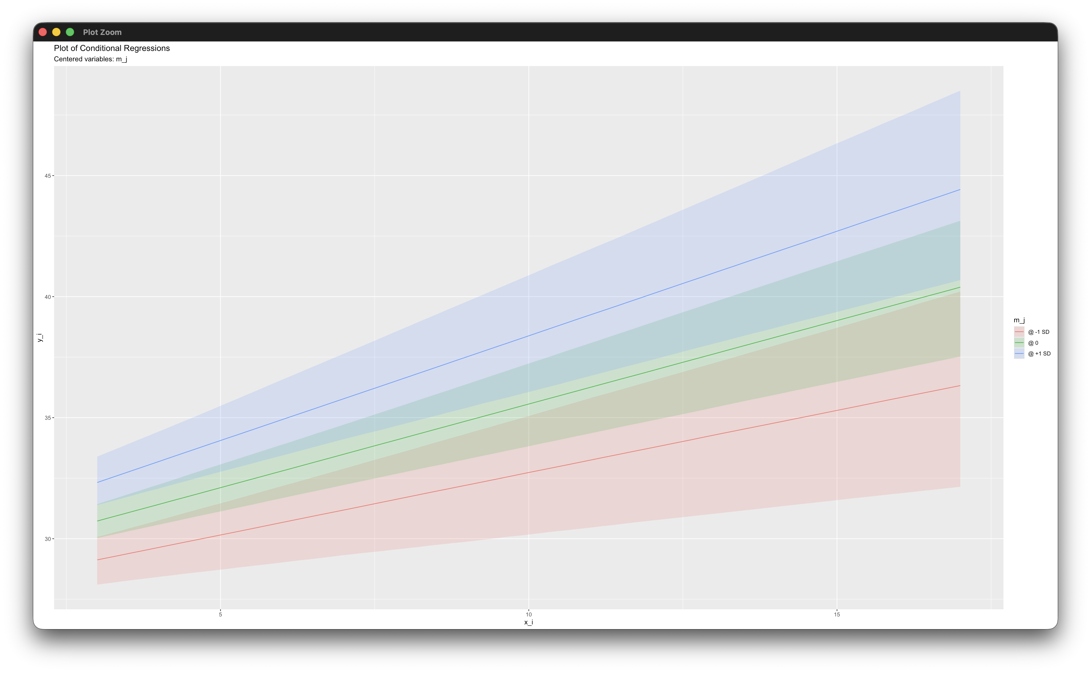
posterior_plot(mymodel)6.11 Cross-Level Interaction Effect
This example illustrates a two-level regression model that includes a cross-level interaction involving a continuous level-1 predictor and a continuous level-2 moderator. The regression model is as follows. The c superscript denotes variables centered at their grand means, and the w (within) superscript denotes variables centered at their level-2 latent group means.
\[y_{ij}=\left(\beta_0+b_{0j}\right)+\left(\beta_1+b_{1j}\right)(x_{ij}^{w})+\beta_2(m_{j}^{c})+\beta_3\left(x_{ij}^{w})(m_{j}^{c}\right)+\varepsilon_{ij}\]
The full set of User Guide examples is available from the Examples pull-down menu in the Blimp Studio graphical interface. A GitHub repository with Blimp Studio scripts and data is available here, and a repository containing the rblimp scripts is available here.
The syntax highlights are listed below.
CLUSTERIDcommand identifies a level-2 identifier, automatically inducing random intercepts for all level-1 variablesCENTERcommand applies grand mean and latent group mean centering to predictorsMODELcommand features a random coefficient listed after the vertical pipeMODELcommand features a product termSIMPLEcommand produces conditional effects (simple slopes) at different standard deviation units of the continuous moderator- Unspecified associations for predictor variables
DATA: data1.dat;
VARIABLES: level1id level2id v1_i v2_i y_i x_i v3_i m_j v4_j;
CLUSTERID: level2id;
MISSING: 999;
CENTER: groupmean = x_i; grandmean = m_j;
MODEL: y_i ~ x_i m_j x_i*m_j | x_i;
SIMPLE: x_i | m_j;
SEED: 90291;
BURN: 10000;
ITER: 10000;
The corresponding rblimp script is as follows.
library(rblimp)

mymodel <- rblimp(
  data = data,
  clusterid = 'level2id',
  center = 'groupmean = x_i;
  grandmean = m_j',
  model = 'y_i ~ x_i m_j x_i*m_j | x_i',
  simple = 'x_i | m_j',
  seed = 90291,
  burn = 10000,
  iter = 10000
)

output(mymodel)
posterior_plot(mymodel,'y_i')
simple_plot(y_i ~ x_i | m_j, mymodel)
Working in rblimp is advantageous because graphing functions are available for visualizing results. For example, the simple_plot function graphs the simple intercepts and slopes for x_i at standard deviation units of the moderator, as shown below.
Alternatively, the analysis can be cast as a multilevel structural equation model. The model setup is similar to Example 6.4. This model does not include an explicit product term. Rather, the cross-level product is represented as a level-2 predictor in the random slope latent variable’s equation. The level-1 and level-2 models are as follows.
\[y_{ij}=\beta_{0j}+\beta_{1j}x_{ij}^{w}+\varepsilon_{ij}\]
\[\beta_{0j}=\beta_{0}+\beta_2m_{j}^{c}+b_{0j}\]
\[\beta_{1j}=\beta_{1}+\beta_3m_{j}^{c}+b_{1j}\]
The script for the multilevel SEM is shown below.
DATA: data1.dat;
VARIABLES: level1id level2id v1_i v2_i y_i x_i v3_i m_j v4_j;
CLUSTERID: level2id;
MISSING: 999;
LATENT: level2id = beta0_j beta1_j;
CENTER: groupmean = x_i; grandmean = m_j;
MODEL:
  level2.model:
  beta0_j ~ 1 m_j;
  beta1_j ~ 1 m_j;
  beta0_j ~~ beta1_j;
  level1.model:
  y_i ~ 1@beta0_j x_i@beta1_j;
SEED: 90291;
BURN: 10000;
ITER: 10000;
The corresponding rblimp script is as follows.
library(rblimp)

mymodel <- rblimp(
  data = data,
  clusterid = 'level2id',
  latent = 'level2id = beta0_j beta1_j',
  center = 'groupmean = x_i;
  grandmean = m_j',
  model = '
    level2.model:
    beta0_j ~ 1 m_j;
    beta1_j ~ 1 m_j;
    beta0_j ~~ beta1_j;
    level1.model:
    y_i ~ 1@beta0_j x_i@beta1_j',
  seed = 90291,
  burn = 10000,
  iter = 10000
)

output(mymodel)
posterior_plot(mymodel)
6.12 1-1-1 Mediation With Random Slopes
This example illustrates a two-level path model that features an indirect effect of two level-1 predictors, both of which are within-cluster centered at their latent group means. The regression models are as follows.
\[x_{ij}=\mu_{x_j}+\varepsilon_{x_{ij}}\]
\[m_{ij}=\mu_{m_j}+\alpha_j(x_{ij} - \mu_{x_j})+\varepsilon_{m_{ij}}\]
\[y_{ij}=\mu_{y_j}+\beta_j(m_{ij} - \mu_{m_j})+\tau^{'}_{j}(x_{ij} - \mu_{x_j})+\varepsilon_{y_{ij}}\]
\[\mu_{x_j}=\mu_x+u_{x_{j}}\]
\[\mu_{m_j}=\mu_m+u_{m_{j}}\]
\[\mu_{y_j}=\mu_y+u_{y_{j}}\]
\[\alpha_j=\mu_{\alpha}+u_{\alpha_{j}}\]
\[\beta_j=\mu_{\beta}+u_{\beta_{j}}\]
\[\tau_j^{'}=\mu_{\tau^{'}}+u_{\tau_{j}^{'}}\]
The random slopes are pure within-cluster effects because the predictors are centered at their latent cluster means. The path diagram below shows the model.

The ellipses in the between-cluster model represent the latent group means (i.e., random intercepts) and random slopes. Note that the α and β random slopes are correlated with each other but all other random effects are independent. This model specification follows Yuan and MacKinnon (2009). The latent variable definitions are the same as those from the multilevel SEM analyses in Example 6.4.
The full set of User Guide examples is available from the Examples pull-down menu in the Blimp Studio graphical interface. A GitHub repository with Blimp Studio scripts and data is available here, and a repository containing the rblimp scripts is available here.
The syntax highlights are listed below.
CLUSTERIDcommand identifies a level-2 identifier, automatically inducing random intercepts for all level-1 variablesLATENTcommand defines between-cluster latent variables representing the random intercepts and slopesMODELcommand uses labels ending in a colon to group models and order their summary tables on the outputMODELcommand estimates the random intercept and slope means, using the->operator to specify means for all variables that do not require labelsMODELcommand sets the intercept of the regression equation equal to the level-2 latent mean (e.g.,x_i ~ 1@xmean_j)MODELcommand centers predictors at their latent group means to obtain pure within-cluster variables (e.g.,x_i - xmean_j)MODELcommand omits the random coefficient listed after the vertical pipeMODELcommand sets the random predictor’s slope equal to the random coefficient (e.g.,(x_i - xmean_j)@alpha_j)MODELcommand specifies the correlation between random slopesPARAMETERScommand uses labeled quantities to compute the product of coefficients estimatorPARAMETERScommand uses the.totalvarfunction to access the variance of the random effects
DATA: data1.dat;
VARIABLES: level1id level2id v1_i y_i m_i x_i v2_i v3_j v4_j;
CLUSTERID:  level2id;
MISSING: 999;
LATENT: level2id = xmean_j mmean_j ymean_j
   alpha_j beta_j tau_j;
MODEL:
  level2.models:
  1 -> xmean_j mmean_j ymean_j tau_j;
  alpha_j ~ 1@alpha_mean;
  beta_j ~ 1@beta_mean;
  alpha_j ~~ beta_j@ab_cor;
  level1.models:
  x_i ~ 1@xmean_j;
  m_i ~ 1@mmean_j (x_i - xmean_j)@alpha_j;
  y_i ~ 1@ymean_j (m_i - mmean_j)@beta_j (x_i - xmean_j)@tau_j;
PARAMETERS:
  ab_cov = ab_cor * sqrt(alpha_j.totalvar * beta_j.totalvar);
  ab = alpha_mean * beta_mean + ab_cov;
SEED: 90291;
BURN: 10000;
ITER: 10000;
The corresponding rblimp script is as follows.
library(rblimp)
mymodel <- rblimp(
data = data,
clusterid = 'level2id',
latent = 'level2id = xmean_j mmean_j ymean_j alpha_j beta_j tau_j',
model = '
level2.models:
1 -> xmean_j mmean_j ymean_j tau_j;
alpha_j ~ 1@alpha_mean;
beta_j ~ 1@beta_mean;
alpha_j ~~ beta_j@ab_cor;
level1.models:
x_i ~ 1@xmean_j;
m_i ~ 1@mmean_j (x_i - xmean_j)@alpha_j;
y_i ~ 1@ymean_j (m_i - mmean_j)@beta_j (x_i - xmean_j)@tau_j',
parameters = '
ab_cov = ab_cor * sqrt(alpha_j.totalvar * beta_j.totalvar);
ab = alpha_mean * beta_mean + ab_cov',
seed = 90291,
burn = 10000,
iter = 10000
)
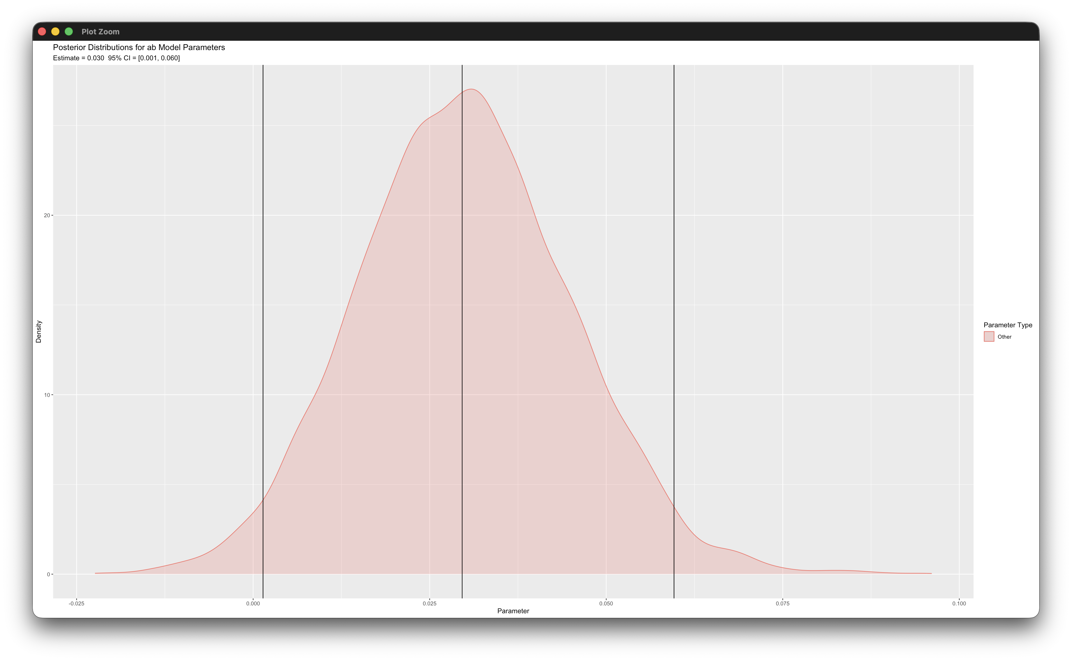
output(mymodel)
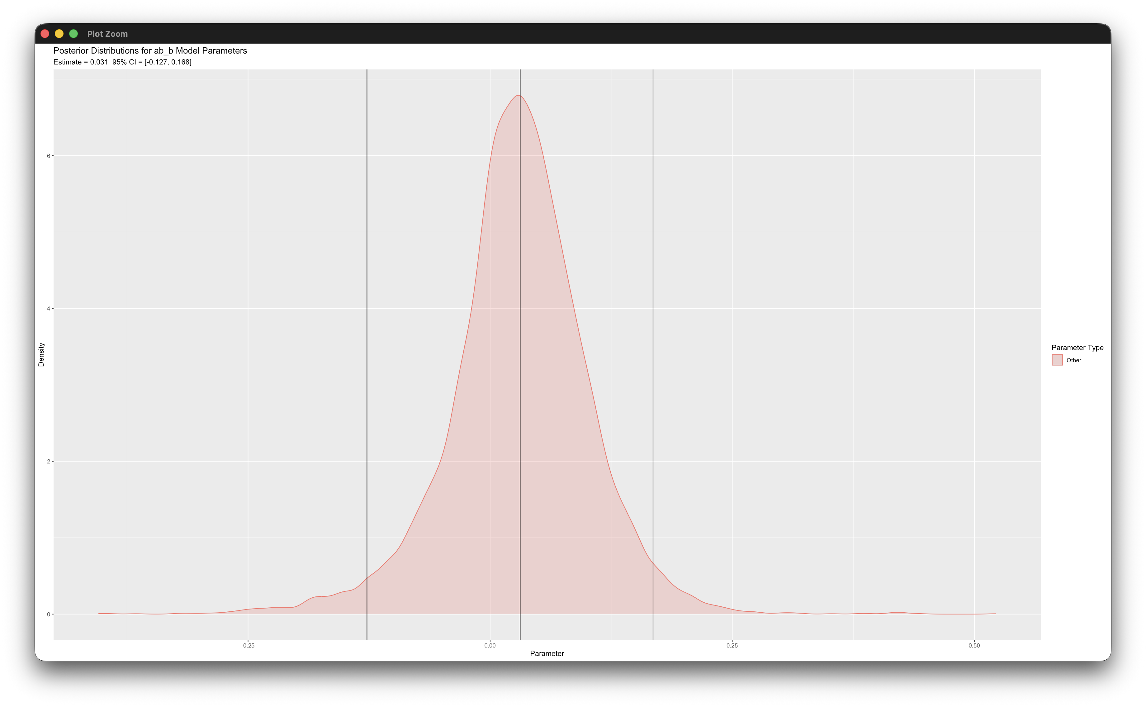
posterior_plot(mymodel,'ab')Working in rblimp is advantageous because graphing functions are available for visualizing results. For example, the posterior_plot function call graphs the distribution of the mediated effect, which is named ab. The 95% intervals are asymmetric because the distribution is skewed, and the graph indicates that the indirect effect is significant because zero is not within the interval.
6.13 1-1-1 Moderated Mediation
This example illustrates a two-level path model that features an indirect effect of two level-1 predictors, both of which are within-cluster centered at their latent group means. A level-2 predictor moderates the α path. Any path can be moderated following the procedures from this example. The model equations are identical to Example 6.12 with two exceptions: the level-2 moderator w_j appears in m_i’s random intercept equation and α’s random slope equation, as follows.
\[\mu_{m_j}=\mu_m+\gamma_1 (w_j)+ u_{m_{j}}\]
\[\alpha_j=\mu_{\alpha}+\gamma_2 (w_j)+u_{\alpha_{j}}\]
The γ2 coefficient captures the cross-level moderation of w_j on the α slope.
The full set of User Guide examples is available from the Examples pull-down menu in the Blimp Studio graphical interface. A GitHub repository with Blimp Studio scripts and data is available here, and a repository containing the rblimp scripts is available here.
The syntax highlights are listed below.
CLUSTERIDcommand identifies a level-2 identifier, automatically inducing random intercepts for all level-1 variablesLATENTcommand defines between-cluster latent variables representing the random intercepts and slopesMODELcommand uses labels ending in a colon to group models and order their summary tables on the outputMODELcommand estimates the random intercept and slope means, using the->operator to specify means for all variables that do not require labelsMODELcommand sets the intercept of the regression equation equal to the level-2 latent mean (e.g.,x_i ~ 1@xmean_j)MODELcommand centers predictors at their latent group means to obtain pure within-cluster variables (e.g.,x_i - xmean_j)MODELcommand omits the random coefficient listed after the vertical pipeMODELcommand sets the random predictor’s slope equal to the random coefficient (e.g.,(x_i - xmean_j)@alpha_j)MODELcommand specifies the correlation between random slopesPARAMETERScommand uses labeled quantities to compute the product of coefficients estimatorPARAMETERScommand uses the.totalvarfunction to access the variance of the random effectsPARAMETERScommand computes the conditional mediated effect at three values of the moderator
DATA: data1.dat;
VARIABLES: level1id level2id v1_i y_i m_i x_i v2_i w_j v3_j;
CLUSTERID:  level2id;
MISSING: 999;
LATENT: level2id = xmean_j mmean_j ymean_j
   alpha_j beta_j tau_j;
CENTER: grandmean = w_j;
MODEL:
  level2.models:
  1 -> xmean_j mmean_j ymean_j tau_j w_j;
  mmean_j ~ w_j;
  alpha_j ~ 1@alpha_mean w_j@product;
  beta_j ~ 1@beta_mean;
  alpha_j ~~ beta_j@ab_cor;
  level1.models:
  x_i ~ 1@xmean_j;
  m_i ~ 1@mmean_j (x_i - xmean_j)@alpha_j;
  y_i ~ 1@ymean_j (m_i - mmean_j)@beta_j (x_i - xmean_j)@tau_j;
PARAMETERS:
  w_stddev = sqrt(w_j.totalvar);
  ab_cov = ab_cor * sqrt(alpha_j.totalvar * beta_j.totalvar);
  ab_low = (alpha_mean - (product * w_stddev)) *
    beta_mean + ab_cov;
  ab_med = alpha_mean * beta_mean + ab_cov;
  ab_high = (alpha_mean + (product * w_stddev)) *
    beta_mean + ab_cov;
SEED: 90291;
BURN: 10000;
ITER: 10000;
The corresponding rblimp script is as follows.
library(rblimp)
mymodel <- rblimp(
data = data,
clusterid = 'level2id',
latent = 'level2id = xmean_j mmean_j ymean_j alpha_j beta_j tau_j',
center = 'grandmean = w_j',
model = '
level2.models:
1 -> xmean_j mmean_j ymean_j tau_j w_j;
mmean_j ~ w_j;
alpha_j ~ 1@alpha_mean w_j@product;
beta_j ~ 1@beta_mean;
alpha_j ~~ beta_j@ab_cor;
level1.models:
x_i ~ 1@xmean_j;
m_i ~ 1@mmean_j (x_i - xmean_j)@alpha_j;
y_i ~ 1@ymean_j (m_i - mmean_j)@beta_j (x_i - xmean_j)@tau_j',
parameters = '
w_stddev = sqrt(w_j.totalvar);
ab_cov = ab_cor * sqrt(alpha_j.totalvar * beta_j.totalvar);
ab_low = (alpha_mean - (product * w_stddev)) *
beta_mean + ab_cov;
ab_med = alpha_mean * beta_mean + ab_cov;
ab_high = (alpha_mean + (product * w_stddev)) *
beta_mean + ab_cov',
seed = 90291,
burn = 10000,
iter = 10000
)
output(mymodel)
posterior_plot(mymodel,'ab_low')
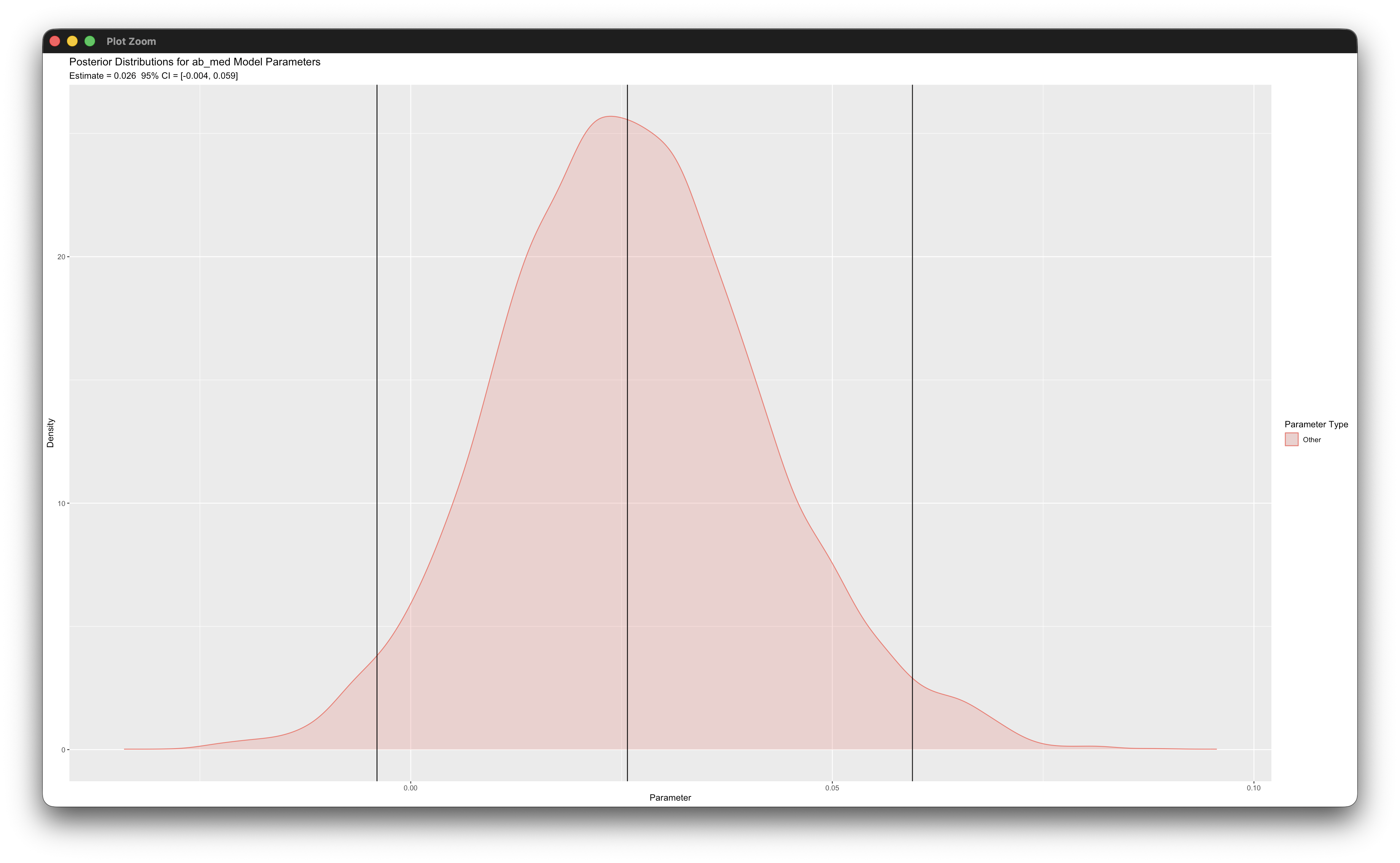
posterior_plot(mymodel,'ab_med')
posterior_plot(mymodel,'ab_high')
posterior_plot(mymodel)Working in rblimp is advantageous because graphing functions are available for visualizing results. For example, the second posterior_plot function call graphs the distribution of the mediated effect at the mean of the moderator, which is named ab_med. The 95% intervals are asymmetric because the distribution is skewed, and the graph indicates that the indirect effect is not significant because zero is within the interval.
6.14 Within- and Between-Level Mediation
This example illustrates a two-level path model that features a within-cluster indirect effect involving centered level-1 variables and a between-cluster indirect effect involving latent group means. The analysis expands on Example 6.12 by specifying directed pathways at level-2. The primary regression models are as follows.
\[x_{ij}=\mu_{x_j}+\varepsilon_{x_{ij}}\]
\[m_{ij}=\mu_{m_j}+\alpha_j(x_{ij} - \mu_{x_j})+\varepsilon_{m_{ij}}\]
\[y_{ij}=\mu_{y_j}+\beta_j(m_{ij} - \mu_{m_j})+\tau^{'}_{j}(x_{ij} - \mu_{x_j})+\varepsilon_{y_{ij}}\]
\[\mu_{x_j}=\mu_x+u_{x_{j}}\]
\[\mu_{m_j}=I_m+\alpha_b(\mu_{x_j})+u_{m_{j}}\]
\[\mu_{y_j}=I_y+\beta_b(\mu_{m_j})+\tau_b^{'}(\mu_{x_j})+u_{y_{j}}\]
\[\alpha_j=\mu_{\alpha}+u_{\alpha_{j}}\]
\[\beta_j=\mu_{\beta}+u_{\beta_{j}}\]
\[\tau_j^{'}=\mu_{\tau^{'}}+u_{\tau_{j}^{'}}\]
The model features distinct within-cluster and between-cluster mediation processes, as depicted in the path diagram below.

The ellipses in the between-cluster model represent latent group means (i.e., random intercepts).
The full set of User Guide examples is available from the Examples pull-down menu in the Blimp Studio graphical interface. A GitHub repository with Blimp Studio scripts and data is available here, and a repository containing the rblimp scripts is available here.
The syntax highlights are listed below.
CLUSTERIDcommand identifies a level-2 identifier, automatically inducing random intercepts for all level-1 variablesLATENTcommand defines between-cluster latent variables representing the random intercepts and slopesMODELcommand uses labels ending in a colon to group models and order their summary tables on the outputMODELcommand estimates the random intercept and slope means, using the->operator to specify means for all variables that do not require labelsMODELcommand sets the intercept of the regression equation equal to the level-2 latent mean (e.g.,x_i ~ 1@xmean_j)MODELcommand centers predictors at their latent group means to obtain pure within-cluster variables (e.g.,x_i - xmean_j)MODELcommand omits the random coefficient listed after the vertical pipeMODELcommand sets the random predictor’s slope equal to the random coefficient (e.g.,(x_i - xmean_j)@alpha_j)MODELcommand specifies the correlation between random slopesPARAMETERScommand uses labeled quantities to compute the product of coefficients estimatorPARAMETERScommand uses the.totalvarfunction to access the variance of the random effects
DATA: data1.dat;
VARIABLES: level1id level2id v1_i y_i m_i x_i v2_i v3_j v4_j;
CLUSTERID:  level2id;
MISSING: 999;
LATENT: level2id = xmean_j mmean_j ymean_j alpha_j beta_j tau_j;
MODEL:
  level2.mediation:
  mmean_j ~ xmean_j@alpha_b;
  ymean_j ~ mmean_j@beta_b xmean_j@tau_b;
  level1.mediation:
  m_i ~ 1@mmean_j (x_i - xmean_j)@alpha_j;
  y_i ~ 1@ymean_j (m_i - mmean_j)@beta_j (x_i - xmean_j)@tau_j;
  level2.models:
  1 -> xmean_j mmean_j ymean_j tau_j;
  alpha_j ~ 1@alpha_mean;
  beta_j ~ 1@beta_mean;
  alpha_j ~~ beta_j@ab_cor;
  level1.models:
  x_i ~ 1@xmean_j;
PARAMETERS:
  ab_cov = ab_cor * sqrt(alpha_j.totalvar * beta_j.totalvar);
  ab_w = alpha_mean * beta_mean + ab_cov;
  ab_b = alpha_b * beta_b;
SEED: 90291;
BURN: 10000;
ITER: 10000;
The corresponding rblimp script is as follows.
library(rblimp)
mymodel <- rblimp(
data = data,
clusterid = 'level2id',
latent = 'level2id = xmean_j mmean_j ymean_j alpha_j beta_j tau_j',
model = '
level2.mediation:
mmean_j ~ xmean_j@alpha_b;
ymean_j ~ mmean_j@beta_b xmean_j@tau_b;
level1.mediation:
m_i ~ 1@mmean_j (x_i - xmean_j)@alpha_j;
y_i ~ 1@ymean_j (m_i - mmean_j)@beta_j (x_i - xmean_j)@tau_j;
level2.models:
1 -> xmean_j mmean_j ymean_j tau_j;
alpha_j ~ 1@alpha_mean;
beta_j ~ 1@beta_mean;
alpha_j ~~ beta_j@ab_cor;
level1.models:
x_i ~ 1@xmean_j',
parameters = '
ab_cov = ab_cor * sqrt(alpha_j.totalvar * beta_j.totalvar);
ab_w = alpha_mean * beta_mean + ab_cov;
ab_b = alpha_b * beta_b',
seed = 90291,
burn = 10000,
iter = 10000
)
output(mymodel)
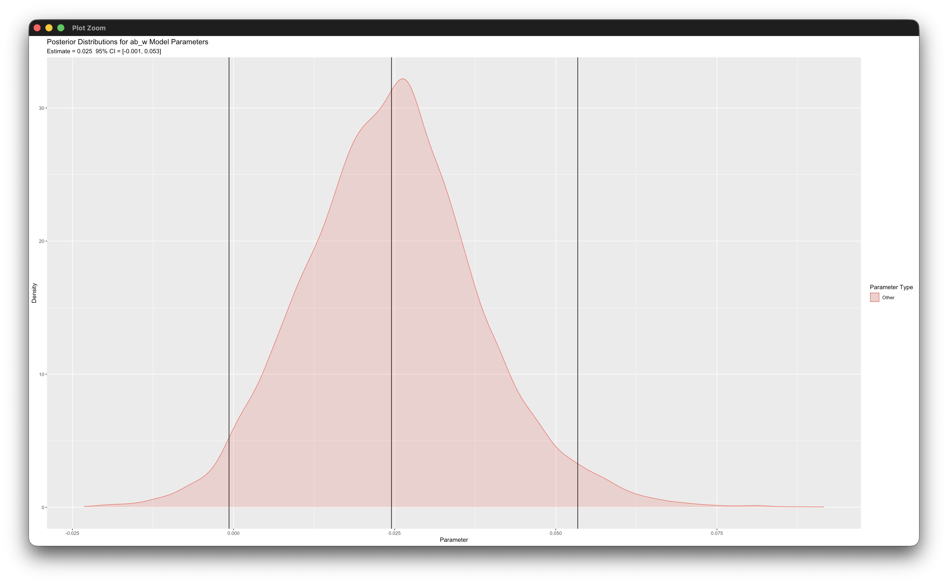
posterior_plot(mymodel,'ab_w')
posterior_plot(mymodel,'ab_b')
posterior_plot(mymodel)Working in rblimp is advantageous because graphing functions are available for visualizing results. For example, the first two posterior_plot function calls graph the distribution of the within- and between-cluster mediated effects, which are named ab_w and ab_b. The 95% intervals are asymmetric because the distribution is skewed. The within-level graph indicates that the indirect effect is not significant because zero is within the interval (although just barely). In the between-level graph, the indirect effect is clearly not significant because zero is near the middle of the interval.
6.15 Two-Level Growth Model
This example illustrates a two-level linear growth model that includes a cross-level group-by-time interaction involving the temporal predictor (time_i = 0, 1, 3, 6) and a binary moderator. The regression model, which is the two-level version of the latent growth model from Example 5.17. The multilevel model features a cross-level (group-by-time) interaction effect involving a level-2 dummy code d_j (e.g., a treatment assignment indicator) and the level-1 time scores, time_i, as follows.
\[y_{ij}=\left(\beta_0+b_{0j}\right)+\left(\beta_1+b_{1j}\right)({time}_{ij})+\beta_2(d_{j})+\beta_3\left({time}_{ij})(d_{j}\right)+\varepsilon_{ij}\]
The full set of User Guide examples is available from the Examples pull-down menu in the Blimp Studio graphical interface. A GitHub repository with Blimp Studio scripts and data is available here, and a repository containing the rblimp scripts is available here.
The syntax highlights are listed below.
CLUSTERIDcommand identifies a level-2 identifier, automatically inducing random intercepts for all level-1 variablesFIXEDcommand identifies complete predictors (optional—speeds computation)NOMINALcommand identifies a binary predictorMODELcommand features a random coefficient listed after the vertical pipeMODELcommand features a product termSIMPLEcommand produces conditional effects (simple slopes) at each level of the nominal moderator
DATA: data9.dat;
VARIABLES: level2id y_i time_i v1_i v2_i v3_i d_j v4_j;
CLUSTERID: level2id;
NOMINAL: d_j;
MISSING: 999;
FIXED: time_i d_j;
MODEL: y_i ~ time_i d_j time_i*d_j | time_i;
SIMPLE: time_i | d_j;
SEED: 90291;
BURN: 10000;
ITER: 10000;
The corresponding rblimp script is as follows.
library(rblimp)
mymodel <- rblimp(
data = data,
clusterid = 'level2id',
nominal = 'd_j',
fixed = 'time_i d_j',
model = 'y_i ~ time_i d_j time_i*d_j | time_i',
simple = 'time_i | d_j',
seed = 90291,
burn = 10000,
iter = 10000
)
output(mymodel)
posterior_plot(mymodel,'y_i')
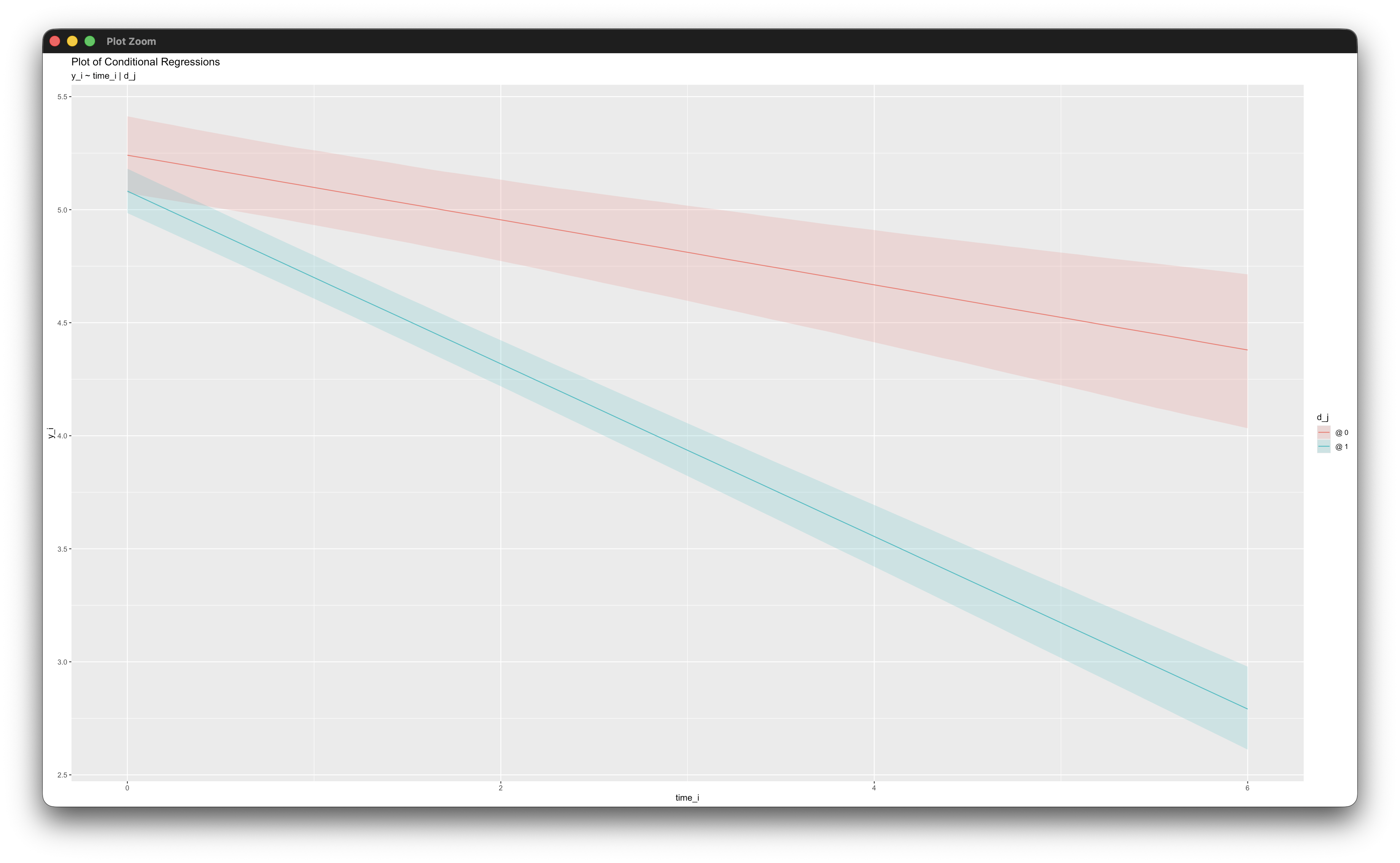
simple_plot(y_i ~ time_i | d_j, mymodel)Working in rblimp is advantageous because graphing functions are available for visualizing results. For example, the simple_plot function graphs of simple intercepts and slopes for each level of d_j, as shown below.
6.16 Three-Level Growth Model
This example illustrates a three-level linear growth model that includes a cross-level group-by-time interaction involving the temporal predictor (time_i = 0, 1, …, 5, 6) and a level-3 binary moderator, d_k. The regression model is as follows.
\[y_{ijk}=\left(\beta_0+b_{0jk}+b_{0k}\right)+\left(\beta_1+b_{1jk}+b_{1k}\right)({time}_{ijk})+\beta_2(d_{k})+\beta_3\left({time}_{ijk})(d_{k}\right)+\varepsilon_{ijk}\]
The full set of User Guide examples is available from the Examples pull-down menu in the Blimp Studio graphical interface. A GitHub repository with Blimp Studio scripts and data is available here, and a repository containing the rblimp scripts is available here.
The syntax highlights are listed below.
CLUSTERIDcommand identifies level-2 and level-3 identifiers (order doesn’t matter), automatically inducing random intercepts for all level-1 and level-2 variablesFIXEDcommand identifies complete predictors (optional—speeds computation)CENTERcommand applies grand mean centering to predictorsNOMINALcommand identifies a binary predictorMODELcommand features a random coefficient listed after the vertical pipeMODELcommand features a product termSIMPLEcommand produces conditional effects (simple slopes) at each level of the nominal moderator
DATA: data10.dat;
VARIABLES: level1id level2id level3id y_i time_i v1_i
   v2_j:v5_j v6_j d_k v7_k v8_k;
NOMINAL: d_k;
CLUSTERID: level2id level3id;
MISSING: 999;
FIXED: time_i d_k;
MODEL: y_i ~ time_i d_k time_i*d_k | time_i;
SIMPLE: time_i | d_k;
SEED: 90291;
BURN: 15000;
ITER: 15000;
The corresponding rblimp script is as follows.
library(rblimp)
mymodel <- rblimp(
data = data,
nominal = 'd_k',
clusterid = 'level2id level3id',
fixed = 'time_i d_k',
model = 'y_i ~ time_i d_k time_i*d_k | time_i',
simple = 'time_i | d_k',
seed = 90291,
burn = 15000,
iter = 15000
)
output(mymodel)
posterior_plot(mymodel,'y_i')
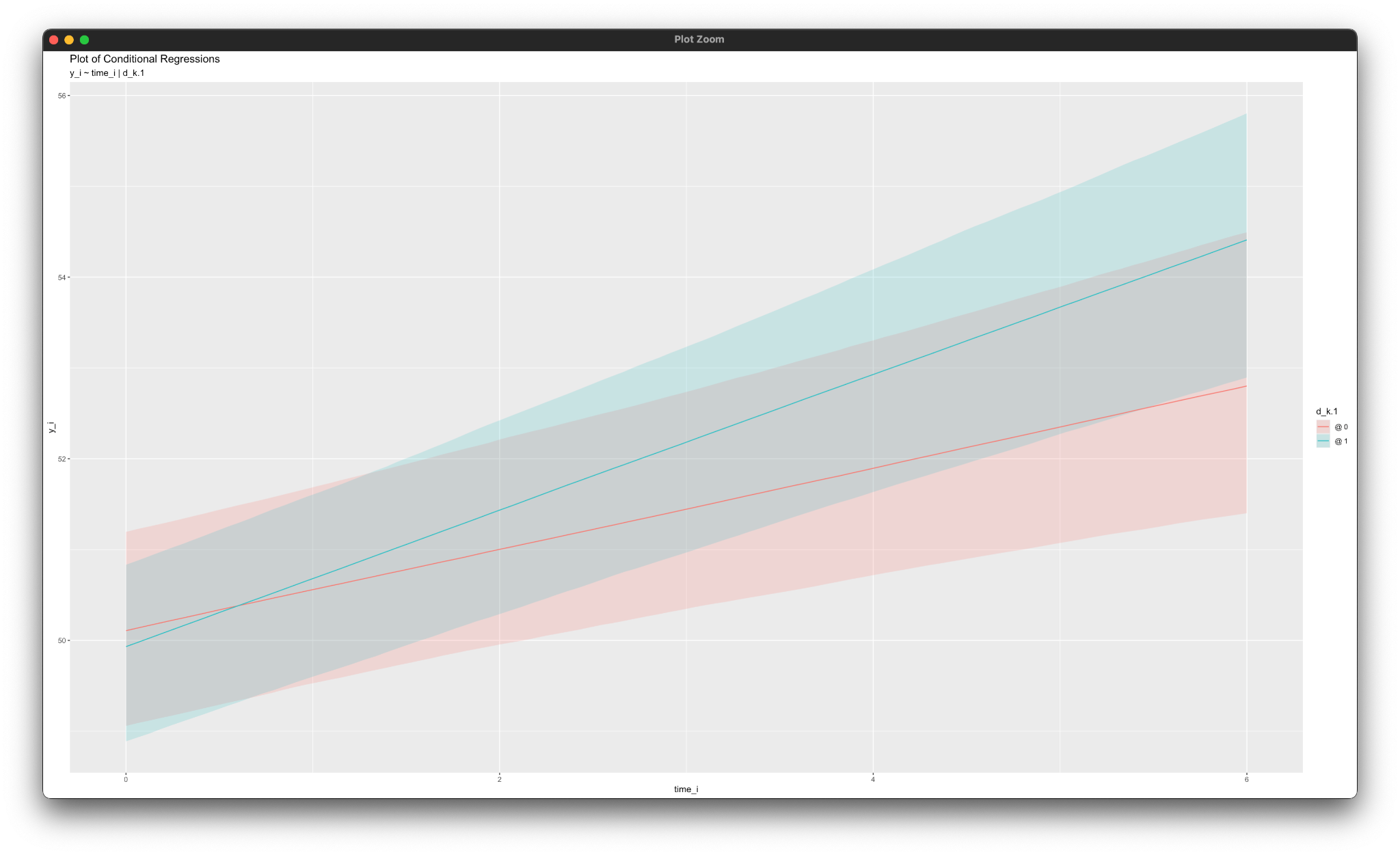
simple_plot(y_i ~ time_i | d_k.1, mymodel)Working in rblimp is advantageous because graphing functions are available for visualizing results. For example, the simple_plot function graphs of simple intercepts and slopes for each level of d_k, as shown below.
By default, Blimp estimates random intercepts and random slopes (when specified) at all levels of the data hierarchy. For example, the previous analysis produces a 2 x 2 covariance matrix of random effects at level-2 and level-3. In some situations, it may be desirable or necessary to override Blimp’s default behavior and fix certain variance components to zero (or alternatively, select which variances get estimated). This is achieved by listing the desired random effects on the right side of the vertical pipe and appending to the effect’s name a cluster-level identifier in square brackets. To illustrate, the following code block illustrates a three-level model with random intercepts at both levels and a random coefficient for the temporal predictor at the second level only.
DATA: data10.dat;
VARIABLES: level1id level2id level3id y_i time_i v1_i
   v2_j:v5_j v6_j d_k v7_k v8_k;
NOMINAL: d_k;
CLUSTERID: level2id level3id;
MISSING: 999;
FIXED: time_i d_k;
MODEL:
  y_i ~ time_i d_k time_i*d_k | 1[level2id] 1[level3id] time_i[level2id];
SIMPLE: time_i | d_k;
SEED: 90291;
BURN: 15000;
ITER: 15000;
The corresponding rblimp script is as follows.
library(rblimp)

mymodel <- rblimp(
  data = data,
  nominal = 'd_k',
  clusterid = 'level2id level3id',
  fixed = 'time_i d_k',
  model = 'y_i ~ time_i d_k time_i*d_k | 1[level2id] 1[level3id] time_i[level2id]',
  simple = 'time_i | d_k',
  seed = 90291,
  burn = 15000,
  iter = 15000
)

output(mymodel)
posterior_plot(mymodel)
6.17 Three-Level SEM Growth Model
This example illustrates a three-level linear growth model that includes a cross-level group-by-time interaction involving the temporal predictor (time_i = 0, 1, …, 5, 6) and a level-3 binary moderator, d_k. The regression model from Example 6.16 is as follows.
\[y_{ijk}=\left(\beta_0+b_{0jk}+b_{0k}\right)+\left(\beta_1+b_{1jk}+b_{1k}\right)({time}_{ijk})+\beta_2(d_{k})+\beta_3\left({time}_{ijk})(d_{k}\right)+\varepsilon_{ijk}\]
This example casts the analysis as a three-level structural equation model. The level-specific equations are as follows.
\[y_{ijk}=\beta_{0jk}+\beta_{1jk}(time_{ijk})+\varepsilon_{ijk}\]
\[\beta_{0jk}=\beta_{0k}+b_{0jk}\]
\[\beta_{1jk}=\beta_{1k}+b_{1jk}\]
\[\beta_{0k}=\beta_{0}+\beta_2(d_k)+b_{0k}\]
\[\beta_{1k}=\beta_{1}+\beta_3(d_k)+b_{1k}\]
The full set of User Guide examples is available from the Examples pull-down menu in the Blimp Studio graphical interface. A GitHub repository with Blimp Studio scripts and data is available here, and a repository containing the rblimp scripts is available here.
The syntax highlights are listed below.
CLUSTERIDcommand identifies level-2 and level-3 identifiers (order doesn’t matter), automatically inducing random intercepts for all level-1 and level-2 variablesORDINALcommand identifies binary predictorFIXEDcommand defines complete predictorsCENTERcommand applies grand mean and latent group mean centering to predictorsLATENTcommand defines two between-cluster latent variables representing the random intercepts and slopesMODELcommand uses labels ending in a colon to group models and order their summary tables on the outputMODELcommand estimates the random intercept and slope meansMODELcommand sets the intercept of the regression equation equal to the level-2 latent mean (i.e.,1@beta0_j)MODELcommand omits the random coefficient listed after the vertical pipeMODELcommand sets the random predictor’s slope equal to the random coefficient (i.e.,x1_i@beta1_j)MODELcommand specifies correlation between random intercepts and random slopes (level-2 latent variables)
DATA: data10.dat;
VARIABLES: level1id level2id level3id y_i time_i v1_i
  v2_j:v5_j v6_j d_k v7_k v8_k;
NOMINAL: d_k;
CLUSTERID: level2id level3id;
MISSING: 999;
LATENT: level2id = beta0_j beta1_j; level3id = beta0_k beta1_k;
MODEL:
  level3.model:
  beta0_k ~ 1 d_k;
  beta1_k ~ 1 d_k;
  beta0_k ~~ beta1_k;
  level2.model:
  beta0_j ~ 1@beta0_k;
  beta1_j ~ 1@beta1_k;
  beta0_j ~~ beta1_j;
  level1.model:
  y_i ~ 1@beta0_j time_i@beta1_j;
SEED: 90291;
BURN: 30000;
ITER: 30000;
The corresponding rblimp script is as follows.
library(rblimp)

mymodel <- rblimp(
  data = data,
  nominal = 'd_k',
  clusterid = 'level2id level3id',
  latent = 'level2id = beta0_j beta1_j;
  level3id = beta0_k beta1_k',
  model = '
    level3.model:
    beta0_k ~ 1 d_k;
    beta1_k ~ 1 d_k;
    beta0_k ~~ beta1_k;
    level2.model:
    beta0_j ~ 1@beta0_k;
    beta1_j ~ 1@beta1_k;
    beta0_j ~~ beta1_j;
    level1.model:
    y_i ~ 1@beta0_j time_i@beta1_j',
  seed = 90291,
  burn = 30000,
  iter = 30000
)

output(mymodel)
posterior_plot(mymodel)
6.18 Two-Level MIMIC Measurement Model
This example illustrates a two-level factor analysis model that features a measurement model for the within-cluster scores at level-1 and the between-cluster latent group means at level-2. The model also features predictor variables at each level, as shown in the path diagram below.

The ellipses in the between-cluster model are latent group means (i.e., random intercepts that load on a level-2 latent variable. The full set of User Guide examples is available from the Examples pull-down menu in the Blimp Studio graphical interface. A GitHub repository with Blimp Studio scripts and data is available here, and a repository containing the rblimp scripts is available here.
The syntax highlights are listed below.
CLUSTERIDcommand identifies a level-2 identifier, automatically inducing random intercepts for all level-1 variablesLATENTcommand defines within- and between-cluster latent variablesMODELcommand uses labels ending in a colon to group models and order their summary tables on the output- Individual regression equations specified for each indicator (instead of the
->convention for latent factors) MODELcommand fixes the within- and between-cluster loading of the first indicator to one- Default specification fixes the latent means equal to zero
DATA: data11.dat;
VARIABLES: level2id y1_i:y4_i x1_i x2_i x3_j;
MISSING: 999;
CLUSTERID: level2id;
LATENT: laty_lev1; level2id = laty_lev2;
CENTER: grandmean = x1_i x2_i x3_j;
MODEL:
  structural.model:
  laty_lev1 ~ x1_i x2_i;
  laty_lev2 ~ x3_j;
  measurement.model:
  y1_i ~ laty_lev1@1 laty_lev2@1;
  y2_i ~ laty_lev1 laty_lev2;
  y3_i ~ laty_lev1 laty_lev2;
  y4_i ~ laty_lev1 laty_lev2;
SEED: 90291;
BURN: 10000;
ITER: 10000;
The corresponding rblimp script is as follows.
library(rblimp)

mymodel <- rblimp(
  data = data,
  clusterid = 'level2id',
  latent = 'laty_lev1;
  level2id = laty_lev2',
  center = 'grandmean = x1_i x2_i x3_j',
  model = '
    structural.model:
    laty_lev1 ~ x1_i x2_i;
    laty_lev2 ~ x3_j;
    measurement.model:
    y1_i ~ laty_lev1@1 laty_lev2@1;
    y2_i ~ laty_lev1 laty_lev2;
    y3_i ~ laty_lev1 laty_lev2;
    y4_i ~ laty_lev1 laty_lev2',
  seed = 90291,
  burn = 10000,
  iter = 10000
)

output(mymodel)
posterior_plot(mymodel)
6.19 Sampling Weights
This example illustrates a two-level regression model with random intercepts and sampling (inverse probability) weights at each level. The regression model is shown below.
\[y_{ij}=\left(\beta_0+b_{0j}\right)+\beta_1x_{1ij}+\beta_2x_{2ij}+\beta_3x_{3ij}+\varepsilon_{ij}\]
Goldstein (2011, Section 3.4.2) describes MCMC estimation for multilevel models with sampling weights. Level-1 and level-2 sampling weights are rescaled following Goldstein (2011, Section 3.4.1). At level-1, the rescaled weights within a given cluster sum to the cluster size. This is the same as the so-called “cluster” method from Asparouhov (2006).
The full set of User Guide examples is available from the Examples pull-down menu in the Blimp Studio graphical interface. A GitHub repository with Blimp Studio scripts and data is available here, and a repository containing the rblimp scripts is available here.
The syntax highlights are as follows.
CLUSTERIDcommand identifies a level-2 identifier, automatically inducing random intercepts for all incomplete level-1 variablesWEIGHTScommand identifies level-1 and level-2 weights (order does not matter)- Unspecified associations for predictor variables
DATA: data21.dat;
VARIABLES: level2id level1wgt level2wgt v1 y_i x1_i x2_i x3_i
   x4_i x5_i;
CLUSTERID: level2id;
WEIGHT: level1wgt level2wgt;
MISSING: 999;
MODEL: y_i ~ x1_i x2_i x3_i;
SEED: 90291;
BURN: 10000;
ITER: 10000;
Note that some data sets may not include level-2 sampling weights, in which case the weight command simplifies as follows.
CLUSTERID: level2id;
WEIGHT: level1wgt;
The corresponding rblimp script is as follows.
library(rblimp)

mymodel <- rblimp(
  data = data,
  clusterid = 'level2id',
  weights = 'level1wgt level2wgt',
  model = 'y_i ~ x1_i x2_i x3_i',
  seed = 90291,
  burn = 10000,
  iter = 10000
)

output(mymodel)
6.20 Partially Nested Design (Singleton Clusters)
This example illustrates a two-level regression model from a partially nested design. The example below considers a level-2 binary predictor (e.g., a treatment assignment indicator) where participants in group d_j = 1 (e.g., treatment participants) are clustered in level-2 units but observations in group d_j = 0 are not nested (i.e., are singleton clusters). The regression model below features an interaction between the binary indicator and the random intercept, such that the random effect term drops from the equation if d_j = 0.
\[y_{ij}=\beta_0+\beta_1d_{j}+d_{j}b_{0j}+\varepsilon_{ij}\]
More generally, the variable d_j does not need to have a fixed effect. Outside of an intervention context, d_j could simply be an indicator that differentiates clustered versus singleton observations (e.g., d_j = 0 is a singleton cluster with a single member, d_j = 1 is an observation that shares cluster membership with other observations). The following random intercept model illustrates this idea.
\[y_{ij}=\beta_0+\beta_1x_{ij}+d_{j}b_{0j}+\varepsilon_{ij}\]
Blimp estimates this model by defining a level-2 latent variable that interacts with d_j. The full set of User Guide examples is available from the Examples pull-down menu in the Blimp Studio graphical interface. A GitHub repository with Blimp Studio scripts and data is available here, and a repository containing the rblimp scripts is available here.
The syntax highlights are as follows.
CLUSTERIDcommand identifies a level-2 identifier, automatically inducing random intercepts for all incomplete level-1 variablesLATENTcommand defines a level-2 latent variable (random intercept), the mean of which is fixed to zero in theMODELsectionMODELcommand eliminates the default random intercept by fixing it to zero (1@0after the vertical pipe)MODELcommand sets the effect ofd_jequal to the the level-2 random intercept
DATA: data19.dat;
VARIABLES: level2id y_i d_j;
MISSING: 999;
CLUSTERID: level2id;
LATENT: level2id = beta0_j;
MODEL:
  beta0_j ~ 1@0;
  y_i ~ d_j d_j@beta0_j | 1@0;
SEED: 90291;
BURN: 10000;
ITER: 10000;
The corresponding rblimp script is as follows.
library(rblimp)

mymodel <- rblimp(
  data = data,
  clusterid = 'level2id',
  latent = 'level2id = beta0_j',
  model = '
    beta0_j ~ 1@0;
    y_i ~ d_j d_j@beta0_j | 1@0',
  seed = 90291,
  burn = 10000,
  iter = 10000
)

output(mymodel)
posterior_plot(mymodel)
Alternatively, the model can be fit as a mixed model by fixing the default random intercept variance to zero and adding the multiple membership dummy indicator as a random slope predictor, as follows.
DATA: data19.dat;
VARIABLES: level2id y_i d_j;
MISSING: 999;
CLUSTERID: level2id;
MODEL: y_i ~ d_j | 1@0 d_j;
SEED: 90291;
BURN: 10000;
ITER: 10000;
The corresponding rblimp script is as follows.
library(rblimp)

mymodel <- rblimp(
  data = data,
  clusterid = 'level2id',
  model = 'y_i ~ d_j | 1@0 d_j',
  seed = 90291,
  burn = 10000,
  iter = 10000
)

output(mymodel)
posterior_plot(mymodel)
6.21 Discrete-Time Survival Model
This example illustrates a discrete-time survival model using Blimp’s multilevel modeling features. The input data set is in stacked (i.e., “person-period”) format with each row representing a time interval nested within an individual. The data also include a set of time indicators that dummy code each measurement interval. The example below illustrates a model with six intervals and thus six dummy codes. The outcome variable is an event indicator that equals 0 if the event did not happen in the interval and a 1 if the event did happen in the interval. Figure 11.5 from Singer and Willett (2003) illustrates the data structure.
The basic model is a logistic regression with the binary event indicator regressed on the time dummy codes.
\[\operatorname{ln}\left(\frac{Pr\left(event=1\right)}{1-Pr\left(event=1\right)}\right)=\alpha_1(t_{1j})+\alpha_2(t_{2j})+\alpha_3(t_{3j})+\alpha_4(t_{4j})+\alpha_5(t_{5j})+\alpha_6(t_{6j})\]
Note that the model omits the usual regression intercept.
The full set of User Guide examples is available from the Examples pull-down menu in the Blimp Studio graphical interface. A GitHub repository with Blimp Studio scripts and data is available here, and a repository containing the rblimp scripts is available here.
The syntax highlights are listed below. Adding the NIMPS and SAVE commands generates imputed data sets, and adding the savepredicted keyword to the OPTIONS command saves predicted probabilities (see Example 4.21).
CLUSTERIDcommand identifies a level-2 identifier, automatically inducing random intercepts for all incomplete level-1 variablesORDINALcommand identifies a binary outcomeFIXEDcommand identifies complete predictors (optional—speeds computation)CENTERcommand applies grand mean centering to predictors- Applying the
logitfunction to the dependent variable on theMODELline requests a logit rather than probit link MODELcommand eliminates the default fixed and random intercepts by fixing both to zero (the1@0after the tilde and vertical pipe)MODELcommand includes Boolean functions that create time-specific dummy codes (e.g.,time_i==1)PARAMETERScommand computes predicted probability of the event at each time point (i.e., hazard probabilities)
DATA: data26.dat;
VARIABLES: level2id time_i y_i d_j x_j;
ORDINAL: y_i;
CLUSTERID: level2id;
MISSING: 999;
FIXED: time_i;
MODEL:
  logit(y_i) ~ 1@0 (time_i==1)@alpha1 (time_i==2)@alpha2
    (time_i==3)@alpha3 (time_i==4)@alpha4 (time_i==5)@alpha5
    (time_i==6)@alpha6 | 1@0;
PARAMETERS:
  hazard.1 = exp(alpha1) / (1 + exp(alpha1));
  hazard.2 = exp(alpha2) / (1 + exp(alpha2));
  hazard.3 = exp(alpha3) / (1 + exp(alpha3));
  hazard.4 = exp(alpha4) / (1 + exp(alpha4));
  hazard.5 = exp(alpha5) / (1 + exp(alpha5));
  hazard.6 = exp(alpha6) / (1 + exp(alpha6));
SEED: 90291;
BURN: 10000;
ITER: 10000;
The corresponding rblimp script is as follows.
library(rblimp)

mymodel <- rblimp(
  data = data,
  ordinal = 'y_i',
  clusterid = 'level2id',
  fixed = 'time_i',
  model = '
    logit(y_i) ~ 1@0 (time_i==1)@alpha1 (time_i==2)@alpha2 (time_i==3)@alpha3
      (time_i==4)@alpha4 (time_i==5)@alpha5 (time_i==6)@alpha6 | 1@0',
  parameters = '
    hazard.1 = exp(alpha1) / (1 + exp(alpha1));
    hazard.2 = exp(alpha2) / (1 + exp(alpha2));
    hazard.3 = exp(alpha3) / (1 + exp(alpha3));
    hazard.4 = exp(alpha4) / (1 + exp(alpha4));
    hazard.5 = exp(alpha5) / (1 + exp(alpha5));
    hazard.6 = exp(alpha6) / (1 + exp(alpha6))',
  seed = 90291,
  burn = 10000,
  iter = 10000
)

output(mymodel)
posterior_plot(mymodel,'y_i')
The next example expands the model by incorporating a person-level dummy code and continuous covariate (d_j and x_j) as predictors of the hazard function. The c superscript denotes grand mean centering.
\[\operatorname{ln}\left(\frac{Pr\left(event=1\right)}{1-Pr\left(event=1\right)}\right)=\alpha_1(t_{1j})+\alpha_2(t_{2j})+\alpha_3(t_{3j})+\alpha_4(t_{4j})+\alpha_5(t_{5j})+\alpha_6(t_{6j})+\beta_1(d_{j})+\beta_2(x_{j}^{c})\]
As before, the model omits the usual regression intercept and includes a set of six dummy codes that index the intervals. The code block below is identical to the previous example, but it defines the binary predictor as ordinal and grand mean centers the continuous covariate.
DATA: data26.dat;
VARIABLES: level2id time_i y_i d_j x_j;
ORDINAL: y_i;
CLUSTERID: level2id;
MISSING: 999;
FIXED: time_i;
CENTER: grandmean = x_j;
MODEL:
  logit(y_i) ~ 1@0 (time_i==1)@alpha1 (time_i==2)@alpha2
    (time_i==3)@alpha3 (time_i==4)@alpha4 (time_i==5)@alpha5
    (time_i==6)@alpha6 d_j x_j | 1@0;
SEED: 90291;
BURN: 10000;
ITER: 10000;
The corresponding rblimp script is as follows.
library(rblimp)

mymodel <- rblimp(
  data = data,
  ordinal = 'y_i',
  clusterid = 'level2id',
  fixed = 'time_i',
  center = 'grandmean = x_j',
  model = '
    logit(y_i) ~ 1@0 (time_i==1)@alpha1 (time_i==2)@alpha2
      (time_i==3)@alpha3 (time_i==4)@alpha4 (time_i==5)@alpha5
      (time_i==6)@alpha6 d_j x_j | 1@0',
  seed = 90291,
  burn = 10000,
  iter = 10000
)

output(mymodel)
posterior_plot(mymodel,'y_i')
6.22 AR(1) Dynamic SEM
This example illustrates an AR(1) dynamic structural equation model (DSEM). The analysis and the data are from McNeish and Hamaker (2020). The application of this model involves intensive repeated measures data nested within persons. The first model features y_i regressed on the “pure” within-cluster components of x_i and the lagged y_i. The variable lag(y_i) is a lagged version of y_i with each person’s data record shifted down by one row and a missing value in the first row (i.e., the first y_i measurement appears in the second row, the second y_i measurement in the third row, and so on). The models below correspond to Equation 4c and Figure 3 in McNeish and Hamaker (2020). We use established generic notation in lieu of their variable names.
The path diagram for the within-person part of the model is shown below. The black dots represent random intercepts and slopes.

The corresponding within-person (level-1) equations are as follows.
\[y_{ij}=\mu_{y_j}+\phi_{j}(\operatorname{lag}(y_{ij})-\mu_{y_j})+\beta_j(x_{ij}-\mu_{x_j})+\varepsilon_{ij}\]
\[x_{ij}=\mu_{x_j}+\epsilon_{ij}\]
Importantly, Blimp does not perform an explicit decomposition of the within- and between-cluster variation. Rather, pure within-person slopes (ϕj and βj) are obtained by centering lag(y_i) and x_i at their level-2 latent group means. Note that lag(y_i) is created using Blimp’s lag function, which works by appending .lag to the variable’s name (e.g., y_i.lag).
The DSEM described in McNeish and Hamaker (2020) and Asparouhov, Hamaker, and Muthén (2018) is different because it uses the residual of y_i rather than the raw y_i as the outcome. However, it is not necessary to explicitly residualize the dependent variable because Blimp’s formulation is mathematically equivalent. The formulation with a residualized outcome is as follows.
\[y_{ij}-\mu_{y_j}=\phi_{j}(\operatorname{lag}(y_{ij})-\mu_{y_j})+\beta_j(x_{ij}-\mu_{x_j})+\varepsilon_{ij}\]
Rearranging the equation to isolate yij on the left-hand side gives the Blimp formulation below.
\[y_{ij}=\mu_{y_j}+\phi_{j}(\operatorname{lag}(y_{ij})-\mu_{y_j})+\beta_j(x_{ij}-\mu_{x_j})+\varepsilon_{ij}\]
Thus, by centering the lagged outcome on the right side of the equation, the model implicitly accounts for the person-mean centered structure without requiring the outcome itself to be centered.
The level-2 model includes the level-2 latent group means of y_i and x_i, μyj and μxj, and the two random slopes, ϕj and βj.
\[\mu_{y_j}=\mu_y+u_{y_j}\]
\[\mu_{x_j}=\mu_x+u_{x_j}\]
\[\phi_j=\mu_{\phi}+u_{\phi_j}\]
\[\beta_j=\mu_{\beta}+u_{\beta_j}\]
Following McNeish and Hamaker (2020), all level-2 random effects are uncorrelated in the example, although they could be correlated. Blimp’s residual correlation diagnostics suggest that random effect correlations should be added, but we follow the original paper’s specification.
The data structure for dynamic structural equation models requires a brief discussion. Blimp’s .lag function assumes that (a) each person has one row of data for every occasion (rows could be filled with missing values), and (b) time scores are discrete and consecutively ordered. For example, the time variable in this example consists of consecutive integers between 1 and 50, and each person has 50 rows of data. If the data do not follow this format, Blimp will automatically restructure the data into time-balanced format using the occasion identifier variable listed on the TIMEID command.
The full set of User Guide examples is available from the Examples pull-down menu in the Blimp Studio graphical interface. A GitHub repository with Blimp Studio scripts and data is available here, and a repository containing the rblimp scripts is available here.
The syntax highlights are listed below.
CLUSTERIDcommand identifies a level-2 identifier, automatically inducing random intercepts for all level-1 variablesTIMEIDcommand identifies variable that indexes time (necessary to compute dropout indicators)LATENTcommand defines between-cluster latent variables representing the random intercepts and slopesMODELcommand uses labels ending in a colon to group models and order their summary tables on the outputMODELcommand estimates the random intercept and slope means, using the->operator to specify means for all variables that do not require labelsMODELcommand sets the intercept of the level-1 regression equation equal to the level-2 latent mean (e.g.,x_i ~ 1@xmean_j)MODELcommand centers predictors at their latent group means to obtain pure within-cluster variables (e.g.,y_i.lag - ymean_j)MODELcommand includes a function to lag the outcome (e.g.,y_i.lag)MODELcommand omits the random coefficient listed after the vertical pipeMODELcommand sets the random predictor’s slope equal to the random coefficient (e.g.,(x_i - xmean_j)@beta_j)
DATA: mcneish_hamaker_2020.dat;
VARIABLES: y_i x_i w1_j w2_j level2id time;
CLUSTERID: level2id;
TIMEID: time;
MISSING: 999;
LATENT: level2id = xmean_j ymean_j phi_j beta_j;
MODEL:
  level2.models:
  1 -> xmean_j ymean_j phi_j beta_j;
  level1.models:
  x_i ~ 1@xmean_j;
  y_i ~ 1@ymean_j (y_i.lag - ymean_j)@phi_j (x_i - xmean_j)@beta_j;
SEED: 90291;
BURN: 20000;
ITER: 20000;
The corresponding rblimp script is as follows.
library(rblimp)

mymodel <- rblimp(
  data = data,
  clusterid = 'level2id',
  timeid = 'time',
  latent = 'level2id = xmean_j ymean_j phi_j beta_j',
  model = '
    level2.models:
    1 -> xmean_j ymean_j phi_j beta_j;
    level1.models:
    x_i ~ 1@xmean_j;
    y_i ~ 1@ymean_j (y_i.lag - ymean_j)@phi_j (x_i - xmean_j)@beta_j;',
  seed = 90291,
  burn = 20000,
  iter = 20000
)

output(mymodel)
The location-scale model allows the within-cluster variance in the y_i model to randomly vary across persons (clusters) and across occasions within persons. Such is the case when people differ with respect to their intraindividual variation. Following Example 6.8, a location-scale model expresses the natural log of the within-cluster variance as a level-2 latent variable (random effect). The mean and variance of this latent variable encode the typical amount of variation and between-cluster differences in the within-cluster variation, respectively (on the logarithmic metric). The scale model has both a within-cluster and between-cluster component, and predictors can be added at each level. The equations below are consistent with Equation 6 from McNeish and Hamaker (2020), but without the predictors (which are added subsequently).
\[\operatorname{ln}(\sigma_{\varepsilon_{j}}^2)=\omega_{0}+u_{\omega_j}\]
A path diagram of the within-person model is shown below. A new latent variable is added representing the logarithm of each person’s intraindividual variation. This latent variable influences the variance of y_i, denoted as a double-headed curved arrow. As before, black dots represent random intercepts and slopes.

We follow the original paper’s specification where all level-2 random effects are uncorrelated, but they can (and often should) be correlated in practice (e.g., intensive repeated measures data often feature random intercepts and random variances that are highly correlated).
Additional syntax highlights are listed below.
MODELcommand includes a variance model for the outcome using thevar(y1_i)functionMODELcommand sets the intercept of the log-variance model equal to the level-2 latent mean (e.g.,var(y1_i) ~ 1@logvar_j)
DATA: mcneish_hamaker_2020.dat;
VARIABLES: y_i x_i w1_j w2_j level2id time;
CLUSTERID: level2id;
TIMEID: time;
MISSING: 999;
LATENT: level2id = xmean_j ymean_j phi_j beta_j logvar_j;
MODEL:
  level2.models:
  1 -> xmean_j ymean_j phi_j beta_j logvar_j;
  level1.models:
  x_i ~ 1@xmean_j;
  y_i ~ 1@ymean_j (y_i.lag - ymean_j)@phi_j (x_i - xmean_j)@beta_j;
  variance.model:
  var(y_i) ~ 1@logvar_j;
SEED: 90291;
BURN: 20000;
ITER: 20000;
The corresponding rblimp script is as follows.
library(rblimp)

mymodel <- rblimp(
  data = data,
  clusterid = 'level2id',
  timeid = 'time',
  latent = 'level2id = xmean_j ymean_j phi_j beta_j logvar_j',
  model = '
    level2.models:
    1 -> xmean_j ymean_j phi_j beta_j logvar_j;
    level1.models:
    x_i ~ 1@xmean_j;
    y_i ~ 1@ymean_j (y_i.lag - ymean_j)@phi_j (x_i - xmean_j)@beta_j;
    variance.model:
    var(y_i) ~ 1@logvar_j;',
  seed = 90291,
  burn = 20000,
  iter = 20000
)

output(mymodel)
A final model extension incorporates time-invariant predictors. The path diagram for the between-person part of the model is shown below.

Importantly, McNeish and Hamaker (2020) assume that all latent variables (random effects are uncorrelated). In our experience, random variances are usually very highly correlated with the outcome’s random intercept. We follow their model setup for this example, noting that we would usually specify random effect correlations.
The script for the expanded analysis is shown below. Note that the intraclass correlation of x_i is very close to zero, which produces low N_eff diagnostics. You could also adopt a slightly informative prior to prevent the variance from collapsing.
DATA: mcneish_hamaker_2020.dat;
VARIABLES: y_i x_i w1_j w2_j level2id time;
CLUSTERID: level2id;
TIMEID: time;
MISSING: 999;
LATENT: level2id = xmean_j ymean_j phi_j beta_j logvar_j;
MODEL:
  level2.models:
  xmean_j ~ 1;
  ymean_j ~ w1_j w2_j xmean_j;
  phi_j ~ w1_j w2_j;
  beta_j ~ w1_j w2_j;
  level1.models:
  x_i ~ 1@xmean_j;
  y_i ~ 1@ymean_j (y_i.lag - ymean_j)@phi_j (x_i - xmean_j)@beta_j;
  variance.model:
  logvar_j ~ 1 w1_j w2_j;
  var(y_i) ~ 1@logvar_j;
SEED: 90291;
BURN: 20000;
ITER: 20000;
The corresponding rblimp script is as follows.
library(rblimp)

mymodel <- rblimp(
  data = data,
  clusterid = 'level2id',
  timeid = 'time',
  latent = 'level2id = xmean_j ymean_j phi_j beta_j logvar_j',
  model = '
    level2.models:
    xmean_j ~ 1;
    ymean_j ~ w1_j w2_j xmean_j;
    phi_j ~ w1_j w2_j;
    beta_j ~ w1_j w2_j;
    level1.models:
    x_i ~ 1@xmean_j;
    y_i ~ 1@ymean_j (y_i.lag - ymean_j)@phi_j (x_i - xmean_j)@beta_j;
    variance.model:
    logvar_j ~ 1 w1_j w2_j;
    var(y_i) ~ 1@logvar_j;',
  seed = 90291,
  burn = 20000,
  iter = 20000
)

output(mymodel)
6.23 VAR(1) Dynamic SEM
This example illustrates a VAR(1) dynamic structural equation model (DSEM). The analysis and the data are from McNeish and Hamaker (2020). The application of this model involves intensive repeated measures data nested within persons. The model features y_i and x_i regressed on the “pure” within-cluster components of the lagged y_i and lagged x_i. The variables lag(y_i) and lag(x_i) are lagged versions of y_i and x_i with each person’s data record shifted down by one row and a missing value in the first row (i.e., the first y_i measurement appears in the second row, the second y_i measurement in the third row, and so on). The models correspond to Equations 7 and 8 and Figure 8 in McNeish and Hamaker (2020). We use established generic notation in lieu of their variable names.
The path diagram for the within-person part of the model is shown below. The black dots represent random intercepts and slopes.

The corresponding within-person (level-1) equations are as follows.
\[y_{ij}=\mu_{y_j}+\phi_{yj}(\operatorname{lag}(y_{ij})-\mu_{y_j})+\beta_{xj}(\operatorname{lag}(x_{ij})-\mu_{x_j})+\varepsilon_{y_{ij}}\]
\[x_{ij}=\mu_{x_j}+\phi_{xj}(\operatorname{lag}(x_{ij})-\mu_{x_j})+\beta_{yj}(\operatorname{lag}(y_{ij})-\mu_{y_j})+\varepsilon_{x_{ij}}\]
Importantly, Blimp does not perform an explicit decomposition of the within- and between-cluster variation. Rather, pure within-person slopes (ϕxj, ϕyj, βxj, and βyj) are obtained by centering lag(y_i) and lag(x_i) at their level-2 latent group means, μyj and μxj. Note that lag(y_i) and lag(x_i) are created using Blimp’s lag function, which works by appending .lag to the variable’s name (e.g., y.lag).
The DSEM described in McNeish and Hamaker (2020) and Asparouhov, Hamaker, and Muthén (2018) is different because it uses the residuals of y_i and x_i rather than the raw y_i and x_i as outcomes. However, it is not necessary to explicitly residualize the variables because Blimp’s formulation is mathematically equivalent. The formulation with residualized outcomes is as follows.
\[y_{ij}-\mu_{y_j}=\phi_{yj}(\operatorname{lag}(y_{ij})-\mu_{y_j})+\beta_{xj}(\operatorname{lag}(x_{ij})-\mu_{x_j})+\varepsilon_{y_{ij}}\]
\[x_{ij}-\mu_{x_j}=\phi_{xj}(\operatorname{lag}(x_{ij})-\mu_{x_j})+\beta_{yj}(\operatorname{lag}(y_{ij})-\mu_{y_j})+\varepsilon_{x_{ij}}\]
Rearranging the equation to isolate yij and xij on the left-hand side of each equation gives the Blimp formulation below.
\[y_{ij}=\mu_{y_j}+\phi_{yj}(\operatorname{lag}(y_{ij})-\mu_{y_j})+\beta_{xj}(\operatorname{lag}(x_{ij})-\mu_{x_j})+\varepsilon_{y_{ij}}\]
\[x_{ij}=\mu_{x_j}+\phi_{xj}(\operatorname{lag}(x_{ij})-\mu_{x_j})+\beta_{yj}(\operatorname{lag}(y_{ij})-\mu_{y_j})+\varepsilon_{x_{ij}}\]
Thus, by centering the lagged variables on the right side of the equation, the model implicitly accounts for the person-mean centered structure without requiring either outcome to be centered.
Following Example 6.22, a location-scale model expresses the natural log of the within-cluster variance as a level-2 latent variable (random effect). The mean and variance of this latent variable encode the typical amount of variation and between-cluster differences in the within-cluster variation, respectively (on the logarithmic metric). The scale models have a within-cluster and between-cluster component, and predictors can be added at each level. The equations below give the level-1 and level-2 parts of the random variation models.
\[\operatorname{ln}(\sigma_{\varepsilon_{yj}}^2)=\omega_{1}+u_{\omega_{1j}}\]
\[\operatorname{ln}(\sigma_{\varepsilon_{xj}}^2)=\omega_{2}+u_{\omega_{2j}}\]
The level-2 model also includes the level-2 latent group means and four random slope coefficients.
\[\mu_{y_j}=\mu_y+u_{y_j}\]
\[\mu_{x_j}=\mu_x+u_{x_j}\]
\[\phi_{yj}=\mu_{\phi_y}+u_{\phi_{yj}}\]
\[\beta_{xj}=\mu_{\beta_x}+u_{\beta_{xj}}\]
\[\phi_{xj}=\mu_{\phi_x}+u_{\phi_{xj}}\]
\[\beta_{yj}=\mu_{\beta_y}+u_{\beta_{yj}}\]
Importantly, McNeish and Hamaker (2020) assume that all latent variables (random effects are uncorrelated). In our experience, random variances are usually very highly correlated with the outcome’s random intercept. We follow their model setup for this example, noting that we would usually specify random effect correlations. Note that the intraclass correlation of x_i is very close to zero. We adopt a slightly informative prior to prevent the variance from collapsing.
The data structure for dynamic structural equation models requires a brief discussion. Blimp’s .lag function assumes that (a) each person has one row of data for every occasion (rows could be filled with missing values), and (b) time scores are discrete and consecutively ordered. For example, the time variable in this example consists of consecutive integers between 1 and 50, and each person has 50 rows of data. If the data do not follow this format, Blimp will automatically restructure the data into time-balanced format using the occasion identifier variable listed on the TIMEID command.
The full set of User Guide examples is available from the Examples pull-down menu in the Blimp Studio graphical interface. A GitHub repository with Blimp Studio scripts and data is available here, and a repository containing the rblimp scripts is available here.
The syntax highlights are listed below.
CLUSTERIDcommand identifies a level-2 identifier, automatically inducing random intercepts for all level-1 variablesTIMEIDcommand identifies variable that indexes time (necessary to compute dropout indicators)LATENTcommand defines between-cluster latent variables representing the random intercepts and slopesMODELcommand uses labels ending in a colon to group models and order their summary tables on the outputMODELcommand estimates the random intercept and slope means, using the->operator to specify means for all variables that do not require labelsMODELcommand sets the intercept of the level-1 regression equation equal to the level-2 latent mean (e.g.,x_i ~ 1@xmean_j)MODELcommand centers predictors at their latent group means to obtain pure within-cluster variables (e.g.,y_i.lag - ymean_j)MODELcommand includes a function to lag the outcome (e.g.,y_i.lag)MODELcommand omits the random coefficient listed after the vertical pipeMODELcommand includes a variance model for the outcome using thevar(y_i)functionMODELcommand sets the intercepts of the log-variance models equal to the level-2 latent means (e.g.,var(y_i) ~ 1@ylogvar_j)MODELcommand sets the random predictor’s slope equal to the random coefficient (e.g.,(x_i - xmean_j)@beta_j)
DATA: mcneish_hamaker_2020.dat;
VARIABLES: y_i x_i w1_j w2_j level2id time;
MISSING: 999;
CLUSTERID: level2id;
TIMEID: time;
LATENT: level2id = xmean_j ymean_j phi_yj beta_xj phi_xj beta_yj logvar_yj logvar_xj;
MODEL:
  level2.models:
  1 -> xmean_j ymean_j phi_yj beta_xj phi_xj beta_yj;
  xmean_j ~~ ymean_j;
  level1.models:
  x_i ~ 1@xmean_j (x_i.lag - xmean_j)@phi_xj (y_i.lag - ymean_j)@beta_yj;
  y_i ~ 1@ymean_j (y_i.lag - ymean_j)@phi_yj (x_i.lag - xmean_j)@beta_xj;
  x_i ~~ y_i;
  variance.model:
  1 -> logvar_yj logvar_xj;
  var(y_i) ~ 1@logvar_yj;
  var(x_i) ~ 1@logvar_xj;
SEED: 90291;
BURN: 20000;
ITER: 20000;
The corresponding rblimp script is as follows.
library(rblimp)

mymodel <- rblimp(
  data = data,
  clusterid = 'level2id',
  timeid = 'time',
  latent = 'level2id = xmean_j ymean_j phi_yj beta_xj phi_xj beta_yj logvar_yj logvar_xj',
  model = '
    level2.models:
    1 -> xmean_j ymean_j phi_yj beta_xj phi_xj beta_yj;
    xmean_j ~~ ymean_j;
    level1.models:
    x_i ~ 1@xmean_j (x_i.lag - xmean_j)@phi_xj (y_i.lag - ymean_j)@beta_yj;
    y_i ~ 1@ymean_j (y_i.lag - ymean_j)@phi_yj (x_i.lag - xmean_j)@beta_xj;
    x_i ~~ y_i;
    variance.model:
    1 -> logvar_yj logvar_xj;
    var(y_i) ~ 1@logvar_yj;
    var(x_i) ~ 1@logvar_xj;',
  seed = 90291,
  burn = 20000,
  iter = 20000
)

output(mymodel)
The syntax can also be streamlined by creating definition variables for the centered predictors and including them in the regression equation as follows.
library(rblimp)

mymodel <- rblimp(
  data = data,
  clusterid = 'level2id',
  timeid = 'time',
  latent = 'level2id = xmean_j ymean_j phi_yj beta_xj phi_xj beta_yj logvar_yj logvar_xj',
  model = '
    level2.models:
    1 -> xmean_j ymean_j phi_yj beta_xj phi_xj beta_yj;
    xmean_j ~~ ymean_j;
    level1.models:
    # definition variables for lags
    xlag_cent = (x_i.lag - xmean_j);
    ylag_cent = (y_i.lag - ymean_j);
    x_i ~ 1@xmean_j xlag_cent@phi_xj ylag_cent@beta_yj;
    y_i ~ 1@ymean_j ylag_cent@phi_yj xlag_cent@beta_xj;
    x_i ~~ y_i;
    variance.model:
    1 -> logvar_yj logvar_xj;
    var(y_i) ~ 1@logvar_yj;
    var(x_i) ~ 1@logvar_xj;',
  seed = 90291,
  burn = 20000,
  iter = 20000
)

output(mymodel)
Other examples of definition variables appear in Examples 5.18 and 5.19.
6.24 Residual (Detrended) Dynamic SEM (RDSEM)
This example illustrates a detrended or residual dynamic structural equation model (RDSEM; Asparouhov, Hamaker, & Muthén, 2018). The analysis and the data are from McNeish and Hamaker (2020). The application of this model involves intensive repeated measures data nested within persons. The model features y_i regressed on the “pure” within-cluster parts of lag of y_i and x_i. The model also includes a linear time trend. The variable lag(y_i) is a lagged version of y_i with each person’s data record shifted down by one row and a missing value in the first row (i.e., the first y_i measurement appears in the second row, the second y_i measurement in the third row, and so on). The model below corresponds to the one described on p. 629 in McNeish and Hamaker (2020). We use established generic notation in lieu of their variable names.
Dynamic structural equation models (DSEMs) for intensive longitudinal data typically assume that the observed scores are stationary, meaning they fluctuate around a stable mean over time. Under this assumption, centering predictors at a person’s latent group mean isolates within-person variation. However, when a systematic time trend exists in the data the scores are no longer mean-reverting and the assumption of stationarity is violated. In such cases, the person’s mean is not constant but rather changes as a function of time, making simple person-mean centering inappropriate. To address this, scores must be “detrended” by computing residuals relative to time-specific predicted values that account for the temporal trend. This detrending process removes the systematic change over time, yielding residuals that reflect genuine within-person fluctuations around the expected trajectory. These residuals can then be used to model autoregressive dynamics, ensuring that the estimated carry-over effects capture true temporal dependencies rather than being confounded with the overall trend in the data. Asparouhov, Hamaker, and Muthén (2018) refer to this as residual DSEM or RDSEM.
The classic two-equation RDSEM first residualizes the outcome based on the covariate and the temporal predictor, and it regresses the residual on the lagged residuals, as follows.
\[y_{ij}=\mu_{y_j}+\beta_{1j}(x_{ij}-\mu_{x_j})+\beta_{2j}(time_{ij})+\zeta_{ij}\]
Notice that the lagged outcome does not appear in this first equation. This is the defining feature of the detrended specification: the autoregression is excluded from the structural (trend) model and instead operates on the residual ζij, which is regressed on its own lag in the second equation below.
\[\zeta_{ij}=\phi_{j}(\operatorname{lag}(y_{ij})-\operatorname{lag}(\hat{y}_{ij}))+\varepsilon_{ij}\]
The lagged predicted value is the outcome score the model expects at the previous occasion, given the person’s mean, the time-varying covariate, and the linear time trend. It is obtained by applying the first equation to the previous occasion.
\[\operatorname{lag}(\hat{y}_{ij})=\mu_{y_j}+\beta_{1j}(\operatorname{lag}(x_{ij})-\mu_{x_j})+\beta_{2j}(time_{i-1,j})\]
Subtracting this expected value from the observed outcome at the previous occasion leaves that occasion’s residual, which is the quantity the autoregression carries forward.
The RDSEM described in McNeish and Hamaker (2020, p. 629) and Asparouhov, Hamaker, and Muthén (2018) is different because it uses the residual of y_i rather than the raw y_i as the outcome. However, it is not necessary to explicitly residualize the dependent variable because Blimp’s formulation is mathematically equivalent. Returning to the RDSEM equations presented above, substituting the second equation into the first gives the single-equation Blimp formation below.
\[y_{ij}=\mu_{y_j}+\phi_{j}(\operatorname{lag}(y_{ij})-\operatorname{lag}(\hat{y}_{ij}))+\beta_{1j}(x_{ij}-\mu_{x_j})+\beta_{2j}(time_{ij})+\varepsilon_{ij}\]
\[\operatorname{lag}(\hat{y}_{ij})=\mu_{y_j}+\beta_{1j}(\operatorname{lag}(x_{ij})-\mu_{x_j})+\beta_{2j}(time_{i-1,j})\]
\[x_{ij}=\mu_{x_j}+\epsilon_{ij}\]
As explained previously, Blimp does not perform an explicit decomposition of the within- and between-cluster variation. Rather, residualized within-person predictors are obtained by centering. In the presence of a time trend, the lagged outcome on the right side of the level-1 regression equation must be centered at its predicted value rather than its latent group mean. The second line defines the predicted value of y_i at the previous time point (i.e., the lag of the predicted values), which accounts for the person’s conditional mean, the effect of the time-varying covariate at that earlier occasion, and the influence of the linear time trend at the previous occasion. By subtracting this predicted value from the lagged y_i, we obtain a detrended residual that isolates genuine within-person fluctuations after removing temporal trends.
The level-2 model includes the level-2 latent group means of y_i and x_i and the three random slopes.
\[\mu_{y_j}=\mu_y+u_{y_j}\]
\[\mu_{x_j}=\mu_x+u_{x_j}\]
\[\phi_j=\mu_{\phi}+u_{\phi_j}\]
\[\beta_{1j}=\mu_{\beta_1}+u_{\beta_{1j}}\]
\[\beta_{2j}=\mu_{\beta_2}+u_{\beta_{2j}}\]
Following McNeish and Hamaker (2020), all level-2 random effects are uncorrelated in the example, although they could be correlated. Blimp’s residual correlation diagnostics suggest that random effect correlations should be added, but we follow the original paper’s specification.
The data structure for dynamic structural equation models requires a brief discussion. Blimp’s .lag function assumes that (a) each person has one row of data for every occasion (rows could be filled with missing values), and (b) time scores are discrete and consecutively ordered. For example, the time variable in this example consists of consecutive integers between 1 and 50, and each person has 50 rows of data. If the data do not follow this format, Blimp will automatically restructure the data into time-balanced format using the occasion identifier variable listed on the TIMEID command.
The full set of User Guide examples is available from the Examples pull-down menu in the Blimp Studio graphical interface. A GitHub repository with Blimp Studio scripts and data is available here, and a repository containing the rblimp scripts is available here.
The syntax highlights are listed below.
CLUSTERIDcommand identifies a level-2 identifier, automatically inducing random intercepts for all level-1 variablesTIMEIDcommand identifies variable that indexes time (necessary to compute dropout indicators)LATENTcommand defines between-cluster latent variables representing the random intercepts and slopesMODELcommand uses labels ending in a colon to group models and order their summary tables on the outputMODELcommand estimates the random intercept and slope means, using the->operator to specify means for all variables that do not require labelsMODELcommand sets the intercept of the level-1 regression equation equal to the level-2 latent mean (e.g.,x_i ~ 1@xmean_j)MODELcommand includes a function to lag the outcome (e.g.,y_i.lag)MODELcommand uses definition variables that specify the residual computations, and it uses those definitions as predictors in the measurement modelsMODELcommand usesifelsefunction to remove the default DSEM prior on the missing outcome score at t = 0MODELcommand omits the random coefficient listed after the vertical pipeMODELcommand sets the random predictor’s slope equal to the random coefficient (e.g.,(x_i - xmean_j)@beta_j)
DATA: mcneish_hamaker_2020_trend.dat;
VARIABLES: y_i x_i w1_j w2_j level2id time;
CLUSTERID: level2id;
TIMEID: time;
MISSING: 999;
LATENT: level2id = ymean_j xmean_j phi_j beta_1j beta_2j;
MODEL:
  # definition variable for the predicted value of y_i.lag
  lag_yhat = ymean_j + (time - 1)*beta_2j + (x_i.lag - xmean_j)*beta_1j;
  # definition variable for residual of y_i.lag, removing default dsem prior at t = 0
  lag_yres = ifelse(time <= 1, 0, y_i.lag - lag_yhat);
  level2.models:
  1 -> ymean_j xmean_j phi_j beta_1j beta_2j;
  level1.models:
  x_i ~ 1@xmean_j;
  y_i ~ 1@ymean_j lag_yres@phi_j (x_i - xmean_j)@beta_1j time@beta_2j;
SEED: 90291;
BURN: 10000;
ITER: 10000;
The corresponding rblimp script is as follows.
library(rblimp)

mymodel <- rblimp(
  data = data,
  clusterid = 'level2id',
  timeid = 'time',
  latent = 'level2id = ymean_j xmean_j phi_j beta_1j beta_2j',
  model = '
    # definition variable for the predicted value of y_i.lag
    lag_yhat = ymean_j + (time - 1)*beta_2j + (x_i.lag - xmean_j)*beta_1j;
    # definition variable for residual of y_i.lag, removing default dsem prior at t = 0
    lag_yres = ifelse(time <= 1, 0, y_i.lag - lag_yhat);
    level2.models:
    1 -> ymean_j xmean_j phi_j beta_1j beta_2j;
    level1.models:
    x_i ~ 1@xmean_j;
    y_i ~ 1@ymean_j lag_yres@phi_j (x_i - xmean_j)@beta_1j time@beta_2j;',
  seed = 90291,
  burn = 10000,
  iter = 10000
)

output(mymodel)
posterior_plot(mymodel)
6.25 Random Effects Meta-Analysis With Known Variances
This example illustrates a random-effects meta-analysis model using Blimp’s multilevel modeling framework. The input data consist of study-level effect size estimates and their corresponding sampling variances, which are treated as known. Each study contributes a single observed effect size, and between-study heterogeneity is modeled through a random effect. The model decomposes variability in the observed effect sizes into within-study sampling error and between-study variation, allowing the overall mean effect to be estimated while accounting for heterogeneity across studies. In this formulation, the sampling variances are fixed and enter the model directly, and the random-effects variance represents unexplained between-study differences in the true effects. This specification corresponds to the conventional random-effects meta-analysis used in many applications, but is implemented here using Blimp’s location-scale model.
In this example, the sampling variances of the study-level effect sizes are treated as known and are incorporated directly into the model. The input data include a variable var_j containing the sampling variance for each study, which is transformed using the natural logarithm. Study-specific variances are incorporated using a location-scale model that fixes the study-specific within-cluster variation from the values in the data. The syntax below fixes the baseline variance term to zero and then uses a series of Boolean expressions of the form (e.g., study == 1) to create study-specific dummy codes. Each dummy code equals 1 for the corresponding study and 0 otherwise, and multiplying these indicators by log-variance acts as an on/off switch that activates the appropriate log-variance value for each study. Fixing the coefficient of each product term to 1 ensures that the variance exactly equals the value supplied in the data. As a result, the model does not estimate sampling variances, but instead treats them as fixed quantities, while still estimating the between-study variance through the random effect. This approach reproduces the conventional random-effects meta-analysis assumption that within-study variances are known.
The full set of User Guide examples is available from the Examples pull-down menu in the Blimp Studio graphical interface. A GitHub repository with Blimp Studio scripts and data is available here, and a repository containing the rblimp scripts is available here.
The syntax highlights are listed below.
CLUSTERIDcommand identifies a level-2 identifier, automatically inducing random intercepts for all level-1 variablesLATENTcommand initializes a level-2 latent variable that represents the random interceptsMODELcommand estimates the latent variable meansMODELcommand sets the intercept of the regression equation equal to the level-2 latent mean (1@beta0_j)MODELcommand omits the random coefficient listed after the vertical pipeMODELcommand includes a variance model for the outcome using thevar()functionMODELcommand sets the intercept of the log-variance model equal to 0, and it fixes the log-variance of each level-2 unit’s within-cluster variance to values from the data (e.g.,(study==1)*log_varj@1)
DATA: effect_sizes.dat;
VARIABLES: study year weeks n1_j n2_j es_j var_j;
TRANSFORM: log_varj = ln(var_j);
MISSING: 999;
CLUSTERID: study;
LATENT: study = beta0_j;
MODEL:
  beta0_j ~ 1;
  es_j ~ 1@beta0_j;
  var(es_j) ~ 1@0 # fix variance of each study to known values
    (study==1)*log_varj@1
    (study==2)*log_varj@1
    (study==3)*log_varj@1
    (study==4)*log_varj@1
    (study==5)*log_varj@1
    (study==6)*log_varj@1
    (study==7)*log_varj@1
    (study==8)*log_varj@1
    (study==9)*log_varj@1
    (study==10)*log_varj@1
    (study==11)*log_varj@1
    (study==12)*log_varj@1
    (study==13)*log_varj@1
    (study==14)*log_varj@1
    (study==15)*log_varj@1
    (study==16)*log_varj@1
    (study==17)*log_varj@1
    (study==18)*log_varj@1
    (study==19)*log_varj@1;
SEED: 90291;
BURN: 10000;
ITER: 10000;
The corresponding rblimp script is as follows.
library(rblimp)

mymodel <- rblimp(
  data = data,
  transform = 'log_varj = ln(var_j)',
  clusterid = 'study',
  latent = 'study = beta0_j',
  model = '
    beta0_j ~ 1;
    es_j ~ 1@beta0_j;
    var(es_j) ~ 1@0 # fix variance of each study
      (study==1)*log_varj@1
      (study==2)*log_varj@1
      (study==3)*log_varj@1
      (study==4)*log_varj@1
      (study==5)*log_varj@1
      (study==6)*log_varj@1
      (study==7)*log_varj@1
      (study==8)*log_varj@1
      (study==9)*log_varj@1
      (study==10)*log_varj@1
      (study==11)*log_varj@1
      (study==12)*log_varj@1
      (study==13)*log_varj@1
      (study==14)*log_varj@1
      (study==15)*log_varj@1
      (study==16)*log_varj@1
      (study==17)*log_varj@1
      (study==18)*log_varj@1
      (study==19)*log_varj@1;',
  seed = 90291,
  burn = 10000,
  iter = 10000
)

output(mymodel)
As described in Chapter 2, BLIMP provides a looping structure within the MODEL command that allows repetitive features of a model more concisely in fewer lines of code (see the Looping Structures section). The MODEL and PARAMETERS section of the script can be specified more concisely as follows.
MODEL:
  beta0_j ~ 1;
  es_j ~ 1@beta0_j;
  var(es_j) ~ 1@0; # fix variance of each study
    { i in 1:19 } : var(es_j) ~ (study==[i])@log_varj;
The loop indexed by i ranges from 1 to 19 and is used to generate study-specific dummy indicators in the variance model. For each value of i, the loop substitutes the index into the expression (study == [i]), automatically creating a separate variance contribution for each study that multiplies the corresponding log-variance predictor log_varj. This looping structure replaces a long sequence of manually written dummy-coded variance terms with a single concise statement.